CBRL and CBRC: Novel Algorithms for Improving Missing Value Imputation Accuracy Based on Bayesian Ridge Regression

Abstract

In most scientific studies such as data analysis, the existence of missing data is a critical problem, and selecting the appropriate approach to deal with missing data is a challenge. In this paper, the authors perform a fair comparative study of some practical imputation methods used for handling missing values against two proposed imputation algorithms. The proposed algorithms depend on the Bayesian Ridge technique under two different feature selection conditions. The proposed algorithms differ from the existing approaches in that they cumulate the imputed features; those imputed features will be incorporated within the Bayesian Ridge equation for predicting the missing values in the next incomplete selected feature. The authors applied the proposed algorithms on eight datasets with different amount of missing values created from different missingness mechanisms. The performance was measured in terms of imputation time, root-mean-square error (RMSE), coefficient of determination (R²), and mean absolute error (MAE). The results showed that the performance varies depending on missing values percentage, size of the dataset, and the missingness mechanism. In addition, the performance of the proposed methods is slightly better.

1. Introduction

Data that contains missing values have been considered as one of the main problems that prevent building an efficient model. Predictive model depends on the quality and size of data; a better quality of data results in a better model accuracy; hence better prediction and analysis. The amount of missing data affects the model performance and produces biased estimates of predictions leading to unacceptable results [1]. The next subsections discuss the types of missingness in data and the handling methods.

1.1. Missingness Mechanisms

Detecting the source of “missingness” is vital, as it affects the selection of the imputation method. The value is missing in three cases: (i) lost or forgotten, (ii) not appropriate to the instance, and (iii) no concern to the instance. For example, missing data occur in the medical field when: (i) the variable was measured, but for an unknown reason the values were not electronically written down, e.g., loss of sensors, errors in connecting with the database server, unintentional human forgetfulness, electricity decay, and others, (ii) the variable was unmeasured all over a quantity of time because of a detectable reason, for instance, the patient was detached from the ventilator as a result of a medical decision, (iii) the variable was unmeasured as it was not related with the patient state and was not offer any clinically valuable info to the specialist [2]. The missingness mechanism (i.e., why there are missing values in data) is well-defined as the association between the probability of being missing and known features [2,3,4,5,6,7,8,9,10]. Mechanisms of missing data are categorised into three types [2,6,11]:

• Missing completely at random (MCAR) [12]: Assume that the missing value indicator matrix $M = \left(M_{ij}\right)$ and the complete data $Y = \left(y_{ij}\right)$. The missing data mechanism is described by the conditional distribution of $M$ given $Y$, say $f(M|Y,\varnothing )$ where $\varnothing$ represents the unknown parameter. If missingness does not depend on the values of the data $Y$, missing or observed, then

  $$f\left(M|Y,\varnothing \right) = f\left(M|\varnothing \right) for all Y,\varnothing$$
• Missing at random (MAR) [12]: Let $Y_{mis}$ and $Y_{obs}$ denote missing data and observed data, respectively. If the Missingness do not depend on the data that are missing, but depends only on $Y_{obs}$ of $Y$, then,

  $$f\left(M|Y,\varnothing \right)=f\left(M|Y_{obs},\varnothing \right) for all Y_{mis},\varnothing$$
• Missing not at random (MNAR) [2]: When the missing data depends on both observed and missing data.

1.2. Dealing with Missing Data

Since most statistical models and data-dependent tool deal only with complete instances; it is important to manipulate data that include missing values. Manipulating missing data can be implemented using deletion (i.e., deleting incomplete instances) or imputation (i.e., substituting any missing values with an assessed value based on the other evidence available) [13].

A deletion may be “complete deletion”, “Complete Case Analysis”, or “list-wise deletion”, wherein all instances involve one or more of their feature values missing are removed. Deletion of the feature which has more than a pre-specified percentage (e.g., 50%) of their feature values missing is called “specific deletion”. In “pair-wise deletion” or “variable deletion”, where the instances involve missing values in the features within the current analysis are removed, these features are used for other studies that do not incorporate the features that contain the missing values. In the worst case of each feature containing missing values across many instances may result in the deletion of the dataset [14]. Statistical methods cannot use the feature if the feature contains missing values; the instance with missing values may still be suitable when analyzing other features with detected values. Pairwise is better than listwise, where it takes into consideration more data. However, statistical analysis can depend on a different subset of the instances; this might be suspicious [1].

Imputation methods benefit from the information available within the dataset to predict the missing value, where the missed value is imputed with a suitable value [14]. Imputation techniques were categorized into two types: intransitive, wherein the imputation of a feature of interest depends on itself, not other features, and transitive, wherein the imputation of a feature of interest depends on other features [15]. Examples of intransitive imputation include the mean, mode, median, and most frequently, examples of transitive imputation include regression and interpolation. Imputation can be implemented in two techniques: multiple imputation and single imputation. Missing values can also be predicted using imputation by hot-deck imputation, K-nearest neighbors (KNNs) and regression methods [11]. The most common methods of linear regression are:

• Simple linear regression: In which a linear relationship between the dependent $y$ and the independent $X$ variables holds

  $$y={\beta }_o+{\beta }_{1}X+\epsilon$$

  (1)

  where ${\beta }_0$ is the value of $y$ when $X$ is equal to zero, ${\beta }_1$ is estimated regression coefficient, and $\epsilon$ is the estimation error.
• Multiple linear regression: In which more independent variables work together to obtain better prediction. The linear relationship between the dependent and independent variables holds

  $$y = {\beta }_o+{\beta }_1{x}_1+{\beta }_2{x}_2+\cdots {\beta }_p{x}_p +\epsilon$$

  (2)

Other models depend on linear regression with additional regularization parameter for the coefficients (e.g., Bayesian Ridge Regression (BRR)). The majority of statisticians and data-dependent tool practitioners prefer to use imputation. Next subsection presents the most relevant imputation algorithms.

1.3. Relevant Imputation Algorithms

This section aims to review some representative and previous published studies that deal with missing data imputation.

K-Nearest Neighbors Imputation (KNNI) is an effective method for manipulating missing data. It firstly looks for the k-most related instances to the missing value in the dataset by calculating the Euclidean distance (K is determined by the user). In the case of a categorical feature involving missing values, then KNNI imputes the missing values within this feature by using the mode of that feature within the k-Nearest Neighbors (k-NN). These k-Nearest neighbors might be found by calculating the Hamming distance for the categorical features. Otherwise, if the feature involving missing data is numerical, the method imputes the missing values within this feature by the mean value of that feature over the k nearest neighbors. KNNI performs better imputation than methods that calculate mode or mean from the whole dataset. KNNI is an effective method that works well on the datasets having a robust local correlation. Nevertheless, KNNI is computationally expensive for large datasets [13,16,17]. Expectation-Maximization-Imputation (EMI) algorithm depends on the covariance matrix and the mean of data to manipulate numerical values that are missing within a dataset. Firstly, the covariance matrix and the mean are calculated from the available information within a dataset, then the missing values are manipulated by the use of the covariance matrix and the mean [13]. Manipulating missing data using fuzzy modeling after a statistical classifier has improved the accuracy of missing values imputation in intensive care units (ICUs) database [12]. Manipulating missing data using some popular methods: complete case analysis, K-nearest neighbor, mean imputation, and median imputation were studied against each other, the comparison was studied on 12 datasets [18]. Dealing with datasets that having missing data via imputation was taken into consideration as an optimization problem. A framework comprising of a support vector machine, decision tree, and K-nearest neighbors was proposed by the authors, choosing the better method from opt.svm, opt.tree, and opt.knn was implemented by opt.cv approach and selecting the better procedure from the iterative mean, predictive-mean matching, Bayesian PCA, and K-nearest neighbors was done by benchmark.cv. Although the proposed framework gives improved results, not only the time for choosing the better methods is long, but also the dimensions of the datasets which have been used by the authors to implement the study were small [3]. Manipulating missing data using fuzzy K-means is a clustering idea and assessment of the accuracy of the algorithm is evaluated in RMSE. The value of the fuzzifier detects whether fuzzy K-means performs better than K-means; this indicates that the fuzzifier value is crucial and must be detected well [19]. Comparing mean, SVM regression, and median was studied in [20], and the experimental studies revealed that SVM has better performance than other methods. The authors did not take into consideration MAE, R² score, or RMSE to assess performance accuracy. In [21], an imputation method that uses an auto-encoder neural network to manipulate missing data was proposed. To train the auto-encoder, two-stage training scheme was used. Eight state-of-the-art imputation methods were compared with the proposed method. In [22], two imputation quantiles-based algorithms were proposed. One of them was done with the help of supplementary information, but the other was not. However, describing the relationship between the feature of concern and the extra feature was an issue. In [5], a genetic algorithm with support vector regression and fuzzy clustering to deal with missing data was proposed. FcmGa, SvrGa, and Zeroimpute methods were compared with the proposed method. Though the proposed method improved the imputation accuracy, the dimension of the whole dataset affects the training stage efficiency, which means that if many features have lots of missing values, lots of instances will be rejected. In [23], the authors proposed an efficient method to impute missing data in classification problems using decision trees. It is very closely related to the approach of dealing with ‘‘missing” as a category in its own exact, generalizing it for use with categorical and continuous features too. Their proposed method showed excellent performance through different collection of data types, and sources and proportions of missingness.

The following sections in this paper are prepared as follows: Section 2 presents the proposed algorithms. Experimental implementation is explained in Section 3. Results and discussion are presented in Section 4. Finally, Section 5 concludes the work.

2. Proposed Algorithms

This section demonstrates the proposed algorithms in detail. BRR is a probabilistic model with a ridge parameter. Ridge regression, in which the Ordinary Least Squares was adjusted to minimize the squared absolute sum of the coefficients, called L2 Regularization. This method is efficient when there is collinearity in your input data features, and ordinary least square will overfit training data. As the proposed algorithms depend on the BRR technique, hence this model is a regression model with additional regularization parameter for the coefficients [24]. The model holds that:

$$y\sim {\rm N}\left(\mu ,\alpha \right)$$

(3)

where:

$$\mu =\beta X= {\beta }_o+{\beta }_1{x}_1+{\beta }_2{x}_2+\cdots {\beta }_p{x}_p$$

$$\beta \sim N\left(0,{\lambda }^{-1}{I}_p\right)$$

$$\alpha \sim ℊ\left({\alpha }_1,{\alpha }_2\right)$$

$$\lambda \sim ℊ\left({\lambda }_1,{\lambda }_2\right)$$

So $y$ follows a Gaussian distribution (the likelihood function) characterized by variance $\alpha$, and mean $\mu = \beta X$. In which gamma priors selected for regularizing parameters $\lambda$ and $\alpha . {\alpha }_1, {\alpha }_2, {\lambda }_1, {\lambda }_2$ are hyper-parameters. The regression parameter $\beta$ has independent Gaussian priors with variance ${\lambda }^{-1} I_p$ and mean zero.

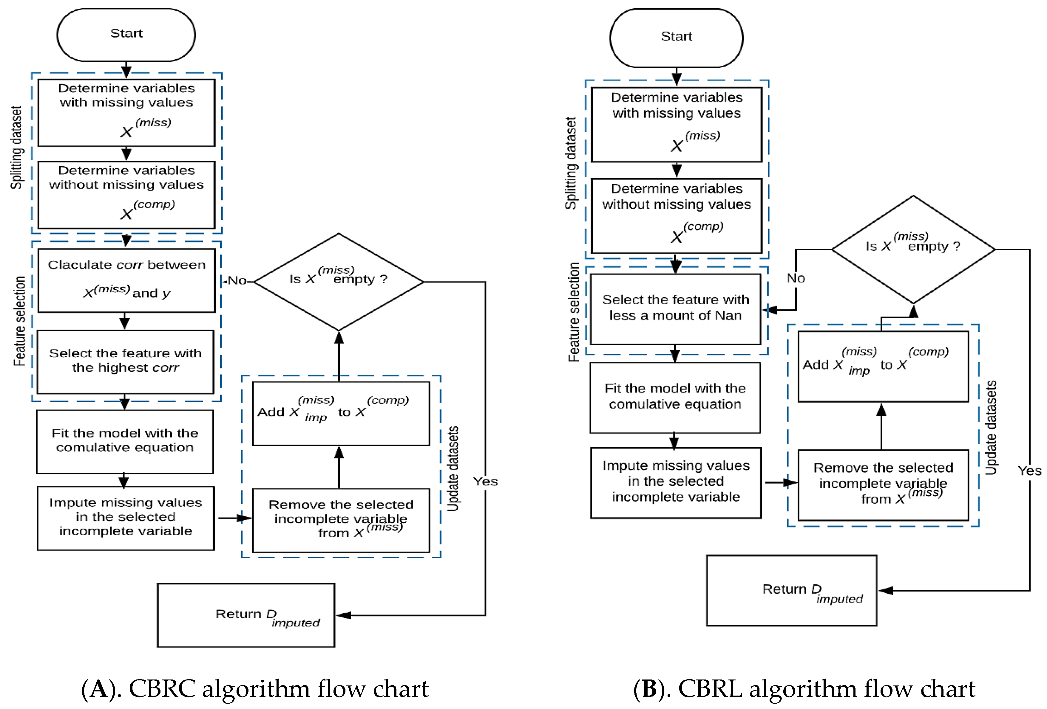
From Figure 1, the following procedural steps provide a more in-depth description of the proposed algorithms:

• In the first step, each proposed algorithm takes a dataset $\mathrm{D}$ as input that holds missing data, then splits it into two sets, the first set $X^{\left(comp\right)}$ includes all complete features, and the second set $X^{\left(mis\right)}$ includes all incomplete features. The authors assume that the target feature $y$ contains no missing data, so $X^{\left(comp\right)}$ comprises all full features plus the target feature $y$.
• In the second step, each proposed algorithm implements its feature selection condition to select the candidate feature to be imputed.
  • The first algorithm, we called Cumulative Bayesian Ridge with Less NaN (CBRL), as its name indicates that this algorithm selects the feature that contains less missing data, which leads the model to be built on the most available information (Algorithm 1).

    Algorithm 1 CBRL

    1: Input: 2:  D: A dataset with missing values containing $n$ instances. 3: Output: 4:  Dimputed: A dataset with all missing features imputed. 5: Definitions: 6:  $X^{\left(comp\right)}$ Set of complete features. 7:  $X^{\left(mis\right)}$ Set of incomplete features. 8:  $X_{imp}^{\left(mis\right) }$ Imputed feature from $X^{\left(mis\right)}$. 9:  $m$ Number of features containing missing values. 10:  $MissObs.X_l^{\left(mis\right) }$ Set of missing instances in the independent feature $X_l^{\left(mis\right) }$ $,l\in \left\{ 1,\dots , m\right\}$. 11:  $Card \left(MissObs.X_l^{\left(mis\right)} \right)$ Number of missing values in the independent feature $X_l^{\left(mis\right) }$. 12: Begin 13:  1 Split D into $X^{\left(comp\right)}$ and $X^{\left(mis\right)}$. 14:  2 From $X^{\left(mis\right)}$ select $X_l^{\left(mis\right)}$ that satisfies the condition: 15:    Min (Card ($MissObs.X_l^{\left(mis\right)}$)). 16:  3 While $X^{\left(mis\right)}$ $\ne \mathsf{Ø}$ 17:    i $g$ ← index of the candidate feature in $X^{\left(mis\right)}$. 18:    ii Fit a Bayesian ridge regression model on $X^{\left(comp\right)}$ as independent features and $X_g^{\left(miss\right)}$ as dependent feature. 19:    iii $X_{imp}^{\left(mis\right) }$ ← Impute the missing data in $X_g^{\left(miss\right)}$ with the fitted model. 20:    iv Delete $X_g^{\left(miss\right)}$ from $X^{\left(mis\right)}$ and add $X_{imp}^{\left(mis\right) }$ to $X^{\left(comp\right)}$. 21:    End While 22:  4 return Dimputed ← $X^{\left(comp\right)}$ 23: End

  • The second algorithm, we called Cumulative Bayesian Ridge with high correlation (CBRC), depends on the highest correlation between the candidate features that contain missing data and the target feature. CBRC chooses the feature that gives the highest correlation with the target feature. The correlation criterion (i.e., Pearson correlation coefficient) is given by Equation (4) [25]:

    $$R\left(i\right) = \frac{cov\left(x_i, Y\right)}{\sqrt{var\left(x_i\right)\ast var\left(Y\right)}}$$

    (4)

    where $x_i$ is the $i\mathrm{th}$ feature, $Y$ is the output feature, $var( )$ is the variance, and $cov( )$ is the covariance. Correlation ranking can only notice linear dependencies between the input feature and output feature (Algorithm 2).

    Algorithm 2 CBRC

    1: Input: 2:  D: A dataset with missing values containing $n$ instances. 3: Output: 4:  Dimputed: A dataset with all missing features imputed. 5: Definitions: 6:  $X^{\left(comp\right)}$ Set of complete features. 7:   $X^{\left(mis\right)}$ Set of incomplete features. 8:  $X_{imp}^{\left(mis\right) }$ Imputed feature from $X^{\left(mis\right)}$. 9:  $m$ Number of features containing missing values. 10:  $Corr \left(X_l^{\left(mis\right)},y\right)$ Correlation between $X_l^{\left(mis\right)}$ and $\mathrm{y}$, $l\in \left\{ 1,\dots , m\right\}$. 11: Begin 11:  1 Split D into $X^{\left(comp\right)}$ and $X^{\left(mis\right)}$. 12:  2 From $X^{\left(mis\right)}$ select $X_l^{\left(mis\right)}$ that satisfies the condition: 13:    Max (Corr ($X_l^{\left(mis\right)},y$)). 14:  3 While $X^{\left(mis\right)} \ne \mathsf{Ø}$ 15:    i $g$ ← index of the candidate feature in $X^{\left(mis\right)}$. 16:    ii Fit a Bayesian ridge regression model on $X^{\left(comp\right)}$ as independent features and $X_g^{\left(miss\right)}$ as dependent feature. 17:    iii $X_{imp}^{\left(mis\right) }$ ← Impute the missing data in $X_g^{\left(miss\right)}$ with the fitted model. 18:    iv Delete $X_g^{\left(miss\right)}$ from $X^{\left(mis\right)}$ and add $X_{imp}^{\left(mis\right) }$ to $X^{\left(comp\right)}$. 19:    End While 20:  4 return Dimputed ← $X^{\left(comp\right)}$ 21: End

• After selecting the candidate feature $X_g^{\left(miss\right)}$, the model is fitted with the cumulative formula defined in Equation (5) using the candidate feature as dependent and the $X^{\left(comp\right)}$ as the independent feature. The selected feature deleted from $X^{\left(mis\right)}$, and after imputation, the imputed feature $X_{imp}^{\left(mis\right) }$ is added to $X^{\left(comp\right)}$. Now $X^{\left(comp\right)}$ consists of all complete features, $y$ and $X_{imp}^{\left(mis\right) }$. Select another candidate feature from $X^{\left(mis\right)}$. Fit the model using the cumulative BRR formula with this candidate feature as the dependent feature and $X^{\left(comp\right)}$ as an independent feature.

  $$X_g^{\left(miss\right)}\sim {\rm N}\left({\mu }_g , {\alpha }_g\right)$$

  (5)

  where:

  $${\mu }_g = {\beta }_o+{\displaystyle \sum }_{i=1}^c{\beta }_i{X}_i^{\left(comp\right)}+{\beta }_{c+1}y+{\displaystyle \sum }_{imp=1}^{g-1}{\beta }_{imp+c+1}{X}_{imp}^{\left(miss\right)2}$$

  $$\beta \sim N\left(0,{\lambda }_g^{-1}{I}_{imp+c+1}\right)$$

  $${\alpha }_g\sim ℊ\left({\alpha }_{1g},{\alpha }_{2g}\right)$$

  $${\lambda }_g\sim ℊ\left({\lambda }_{1g},{\lambda }_{2g}\right)$$

  where $g = 1,2,\dots ,m.$ $m$ is the number of features containing missing values and $c$ is the number of complete independents.
• Repeat from step 2 of feature selection until $X^{\left(mis\right)}$ is empty, then return the imputed dataset ($X^{\left(comp\right)}$), see Figure 1.

3. Experimental Implementation

3.1. Benchmark Datasets

Eight datasets that are commonly used in different databases repository and literature are used in the comparative study. Because of the massive number of instances in Poker Hand and BNG_heart_statlog datasets, randomly sampled sub-datasets of 10,000, 15,000, 20,000, and 50,000 instances of them were used. In each dataset, the missing values were generated in the three types of mechanisms, MAR, MCAR, and MNAR, each with 10%, 20%, 30%, and 40% missingness ratios using R function named ampute [26]. Diabetes dataset is used to predict whether a patient has diabetes or not, depend on certain diagnostic measurements contained in the dataset. Graduate Admissions dataset contains many parameters which are used during the application for Masters Programs for prediction of Graduate Admissions. Profit Estimation dataset is used for prediction of which companies to invest. Red & White Wine dataset contains red and white wine samples. The inputs contain objective tests, and the target is based on sensory data. Each expert graded the quality of the wine between 10 (very excellent) and 0 (very bad). California dataset is used to predict the houses’ price in California in 1990 based on a number of predictors, including longitude information about surrounded houses within a particular block, and latitude. Diamonds dataset includes the prices and other features of almost 54,000 diamonds. It is used to build a predictive model to predict whether a given diamond is a rip-off or a good deal. Poker Hand dataset consists of 1,025,010 records, each record in this dataset includes five playing cards and a feature representing the poker hand. BNG_heart_statlog dataset contains 1,000,000 records and 14 features (13 of them are numeric features and one is nominal feature). The datasets’ specifications are described in

Table 1. Datasets’ specifications. The first column presents the dataset name, the second column presents the number of instances, the third column presents the number of features, and the fourth column presents the missingness mechanism.

Dataset name	#Instances	#Features	Missingness Mechanism
			MAR	MCAR	MNAR
Diabetes [27]	442	11	√	√	√
graduate admissions [28]	500	8	√	√	√
profit estimation of companies [29]	1000	6	√	√	√
red & white wine [30]	4898	12	√	√	√
California [31]	20,640	9	√	√	√
Diamonds [32]	53,940	10	√	√	√
Poker Hand [33]	1,025,010	11	√	√	√
BNG_heart_statlog [34]	1,000,000	14	√	√	√

.

3.2. Evaluation

The imputation algorithm is considered to be efficient if it imputes in a short time with high accuracy and small error. The proposed algorithms were compared with six common imputation algorithms explained briefly in

Table 2. The algorithms used in the comparison.

Method Name	Function Name	Package	Description
MICE [9,26]	mice	impyute	implements the multivariate imputation by chained equations algorithm.
least squares (LS) [35]	SingleImputer	autoimpute	produces predictions using the least squares methodology.
norm [35]	SingleImputer	autoimpute	creates a normal distribution using the sample variance and mean of the detected data.
stochastic (ST) [35]	SingleImputer	autoimpute	samples from the regression’s error distribution and adds the random draw to the prediction.
Fast KNN (FKNN) [36]	fast_knn	impyute	uses K-Dimensional tree to find k nearest neighbor and imputes using the weighted average of them.
EMI [36]	em	impyute	imputes using Expectation-Maximization-Imputation.

. Multiple Imputation by Chained Equations (MICE) is an informative and robust method for handling missing data. The method uses an iterative series of predictive models to impute missing data. Each specified feature in each iteration in the dataset is filled using the other features. These iterations should be repeated until the convergence occurs. Least squares method uses least squares methodology which is a standard method in the regression analysis. It minimizes the sum of squared residuals (i.e., the difference between the fitted value given by a model and the observed value). The norm method constructs a normal distribution using the sample variance and mean of the observed data. The method then randomly samples from this distribution to fill missing data. The stochastic method predicts missing values using the least squares methodology. It then samples from the regression’s error distribution and adds the random draw to the prediction. This method can be used directly, but such behavior is frustrating. Fast KNN method imputes array with a passed in initial impute fn (mean impute) and then use the resulting complete array to construct a KDTree which will be used to compute nearest neighbours. The weighted average of the ‘k’ nearest neighbours will be taken. To compare and evaluate the performance of the proposed algorithms and the other stated methods. The performance evaluation was measured from the point of view of RMSE, MAE, R² score, and the time of imputation in seconds (t). The performance evaluation was calculated for the four missingness ratios.

3.2.1. RMSE and MAE

RMSE and MAE have been used as statistical metrics to assess the performance of the models [37]. RMSE and MAE are defined in Equations (6) and (7) respectively [1].

$$RMSE = \sqrt{\frac{1}{n} {{\displaystyle \sum }}_{l=1}^n{\left( y_l-\widehat{y_l} \right)}^2}$$

(6)

$$MAE = \frac{1}{n}{\displaystyle \sum }_{l=1}^n\left|y_l-\widehat{y_l}\right|$$

(7)

where $y_l$ and $\widehat{y_l}$ are the real value and predicted value of the $lth$ instance respectively, and $n$ is the number of the instances.

3.2.2. R² Score

R² score (Equation (8)) is a statistical measure that indicates how well the predicted values are close to the real data values.

$$R^2\left( y, \widehat{y} \right)=1 - \frac{{{\displaystyle \sum }}_{i=1}^n{\left(y_l-\widehat{y_i}\right)}^2}{{{\displaystyle \sum }}_{l=1}^n{\left(y_l-\overline{y}\right)}^2}$$

(8)

where:

$$\overline{y}= \frac{1}{n}{\displaystyle \sum }_{l=1}^n{y}_l$$

4. Results and Discussion

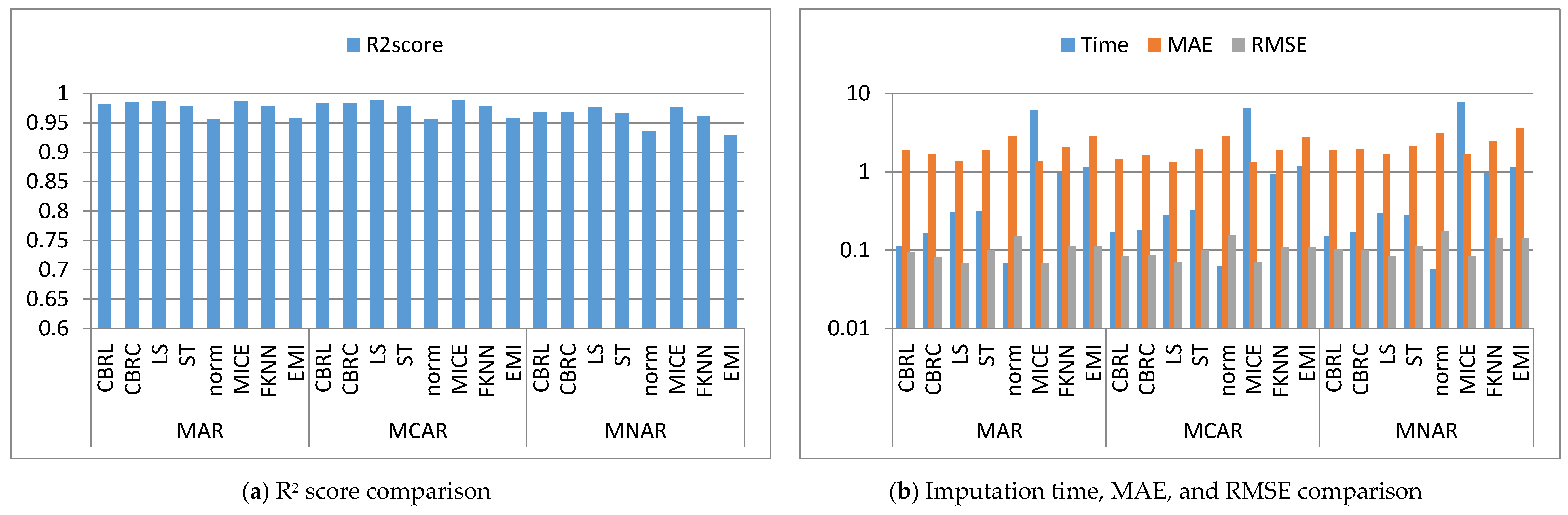
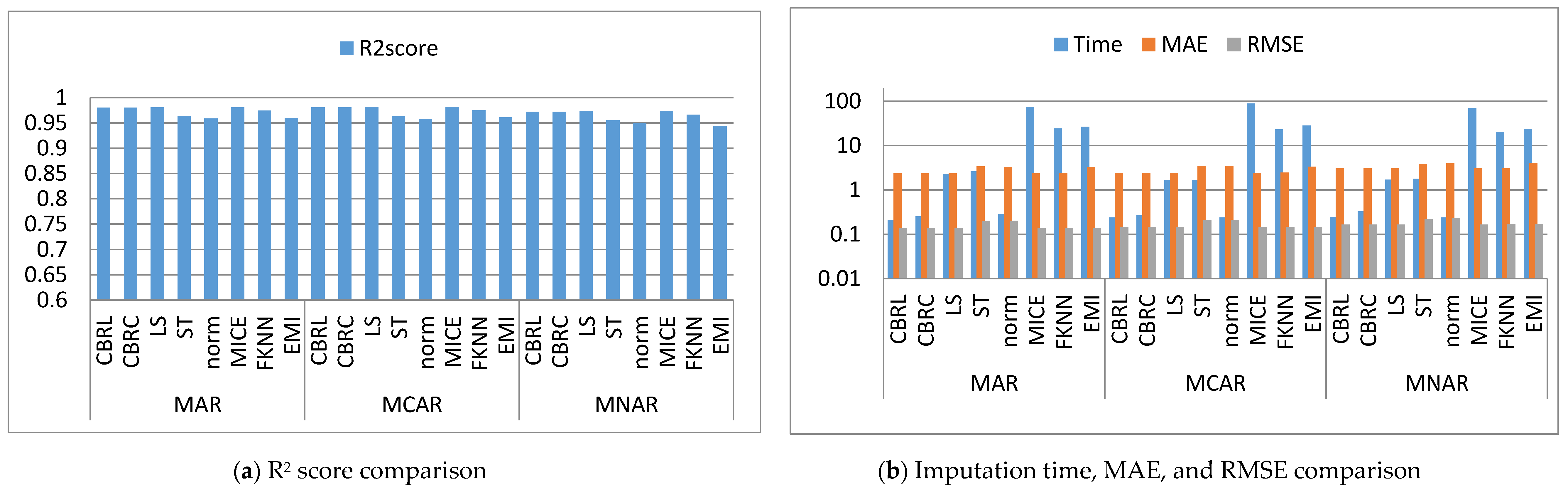
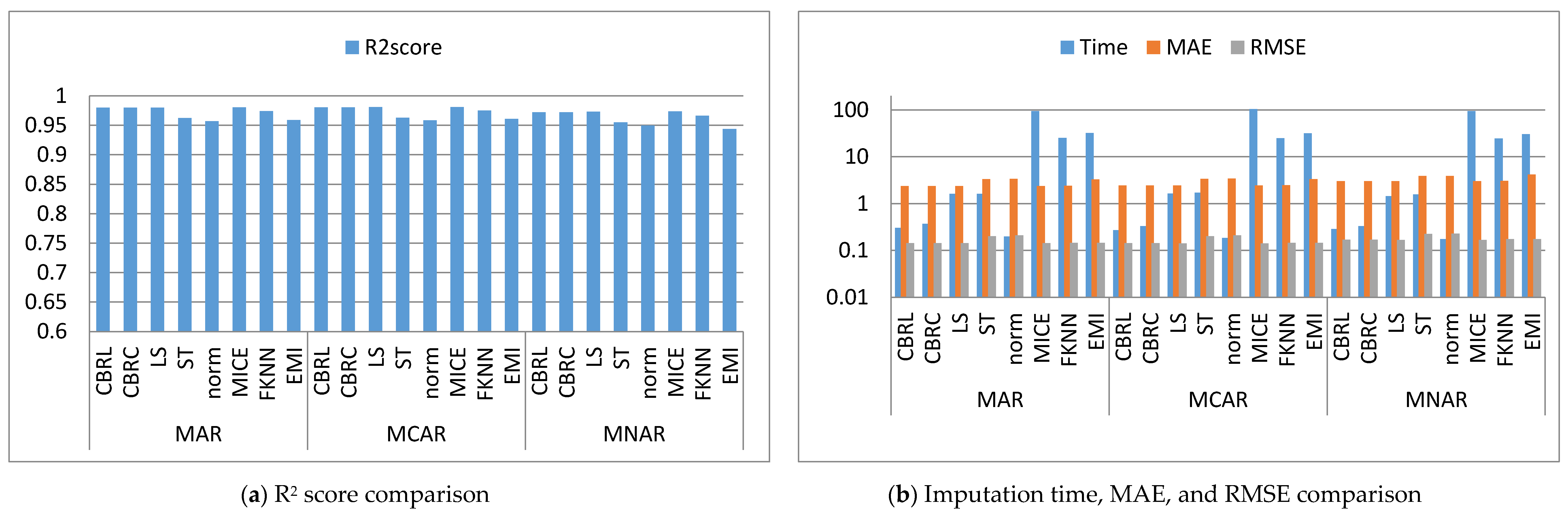
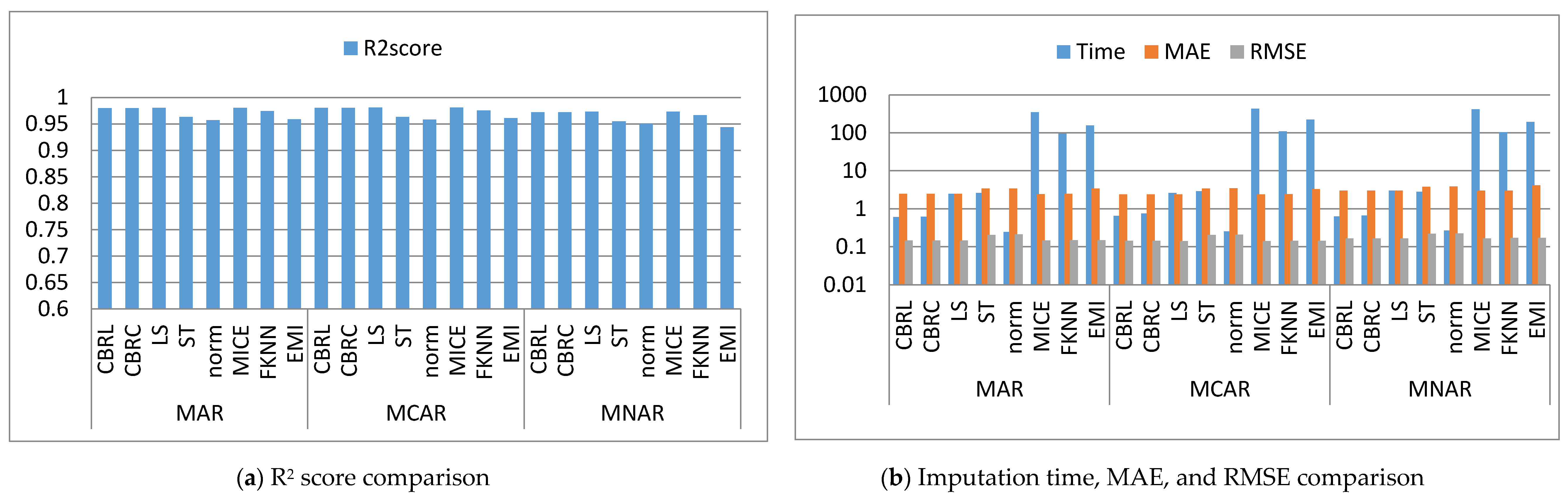
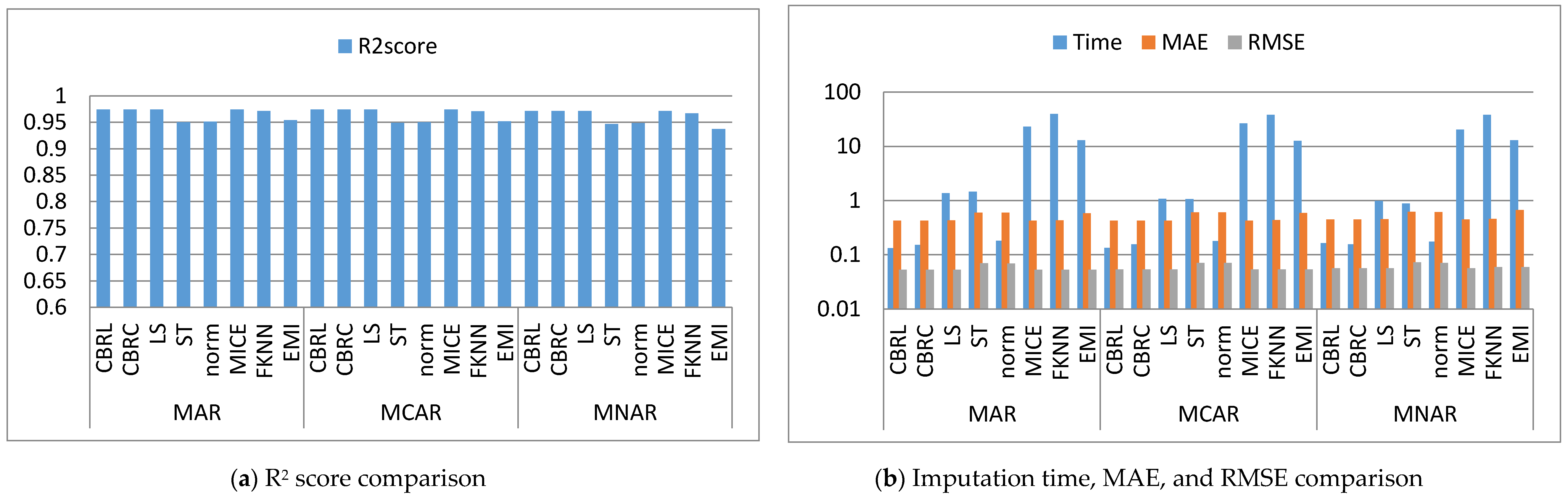
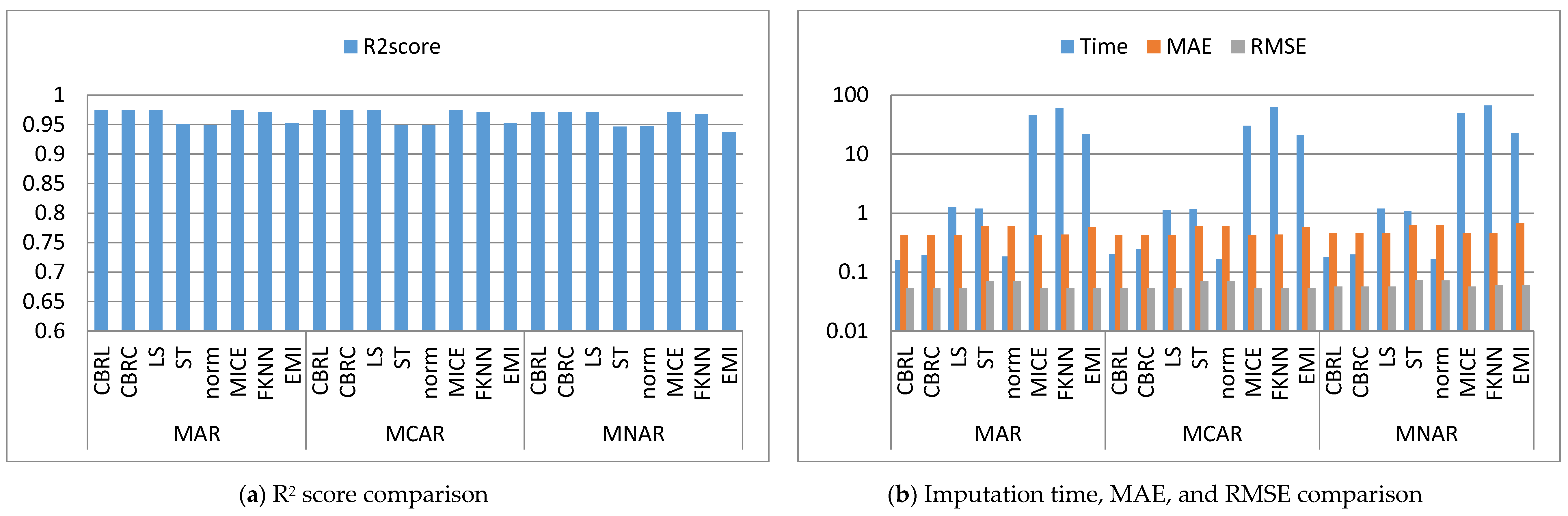
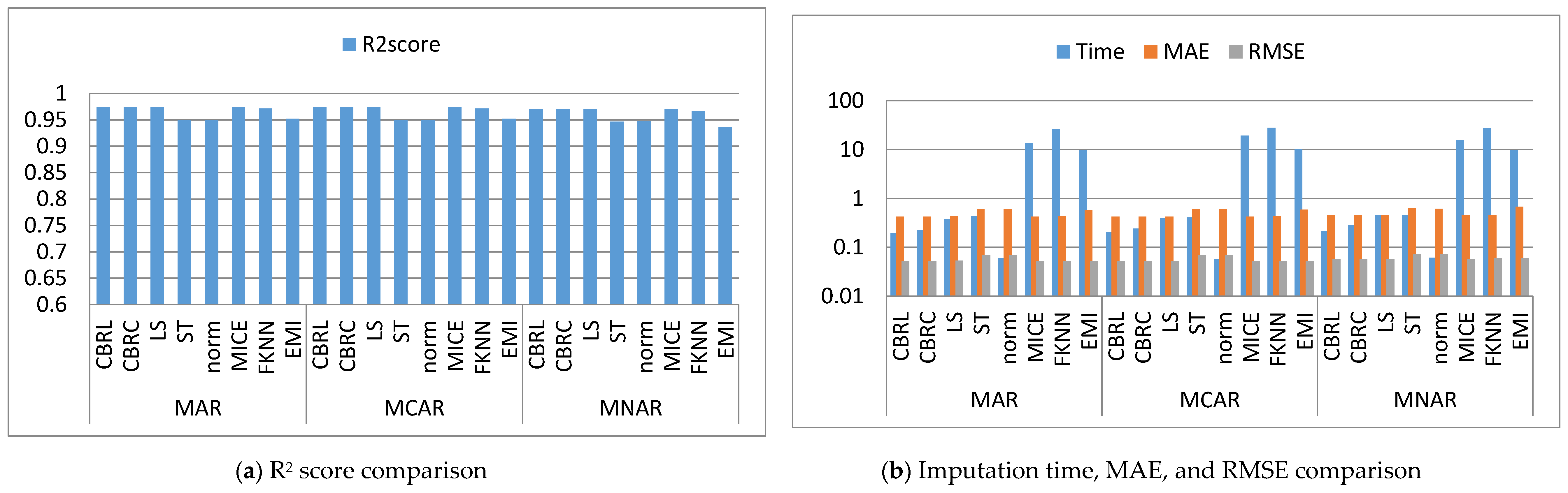
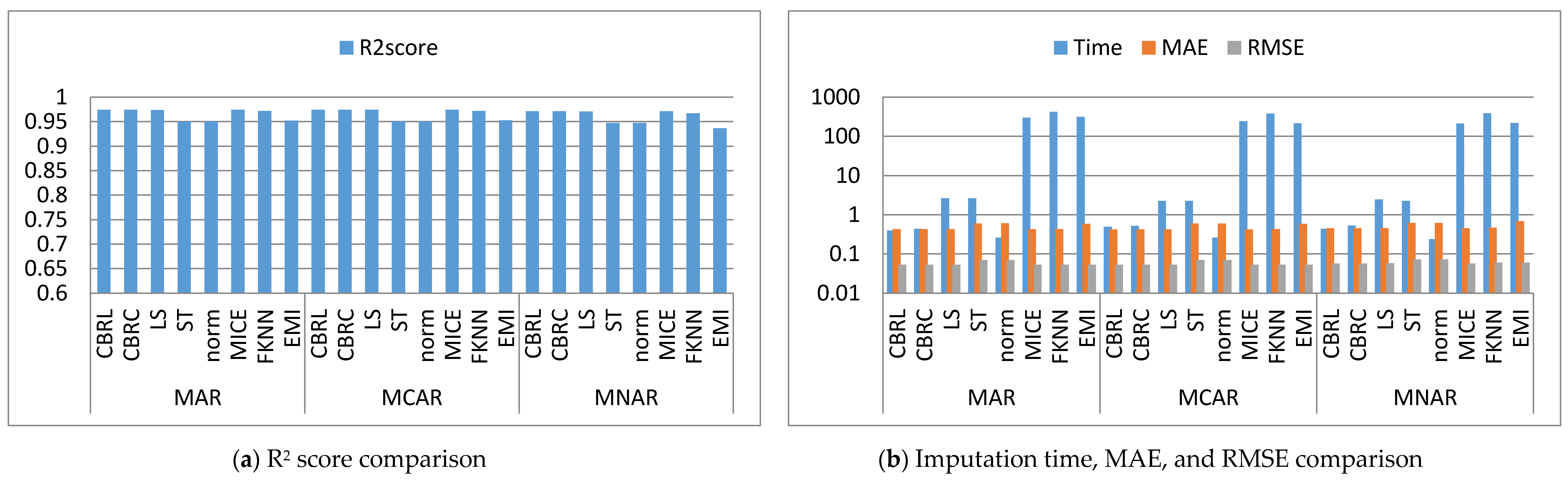
Figure 2, Figure 3, Figure 4, Figure 5, Figure 6, Figure 7, Figure 8, Figure 9, Figure 10, Figure 11, Figure 12, Figure 13, Figure 14 and Figure 15 show the averages of the four evaluation metrics. The figures show that the performance varies depending on the missingness mechanisms, size of the dataset, and missing values proportion. This section is divided into three subsections; the first subsection presents error analysis, the second subsection exhibits the imputation time, and finally, the third subsection presents the performance accuracy. Log scale is used in RMSE, MAE, and imputation time comparisons because each of which has a different range of values. With regard to RMSE, MAE, and imputation time metrics, lower value is better, so they are gathered in the same figure. The computational complexity of both CBRL and CBRC is O(n).

4.1. Error Analysis

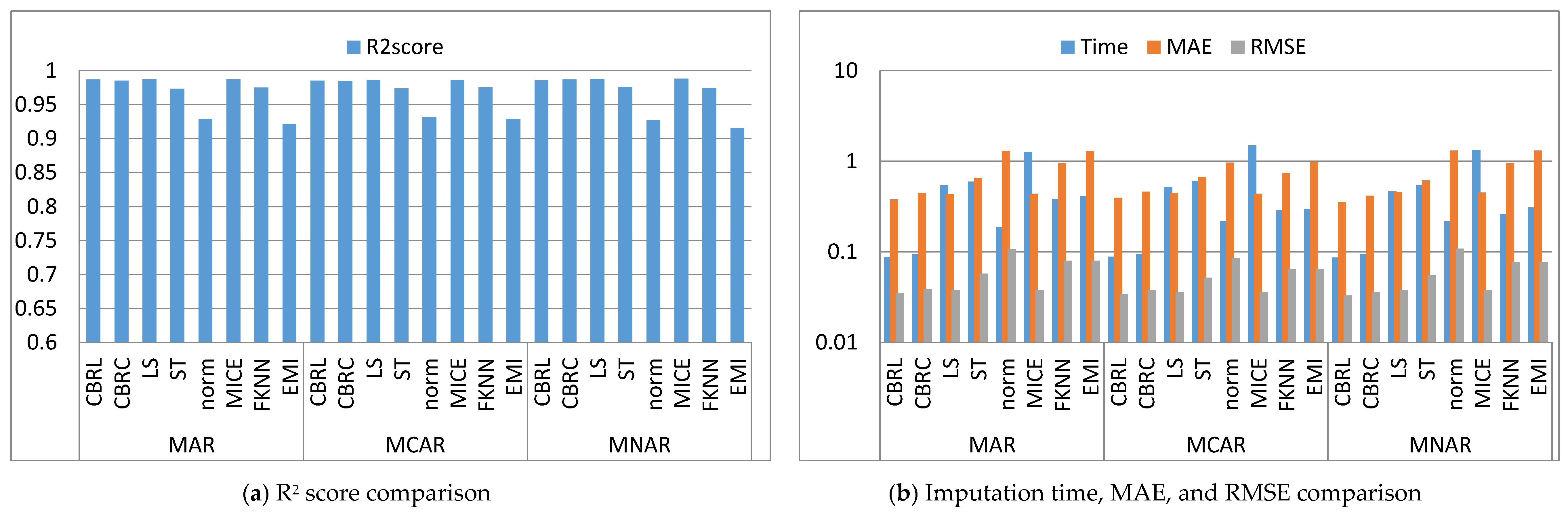
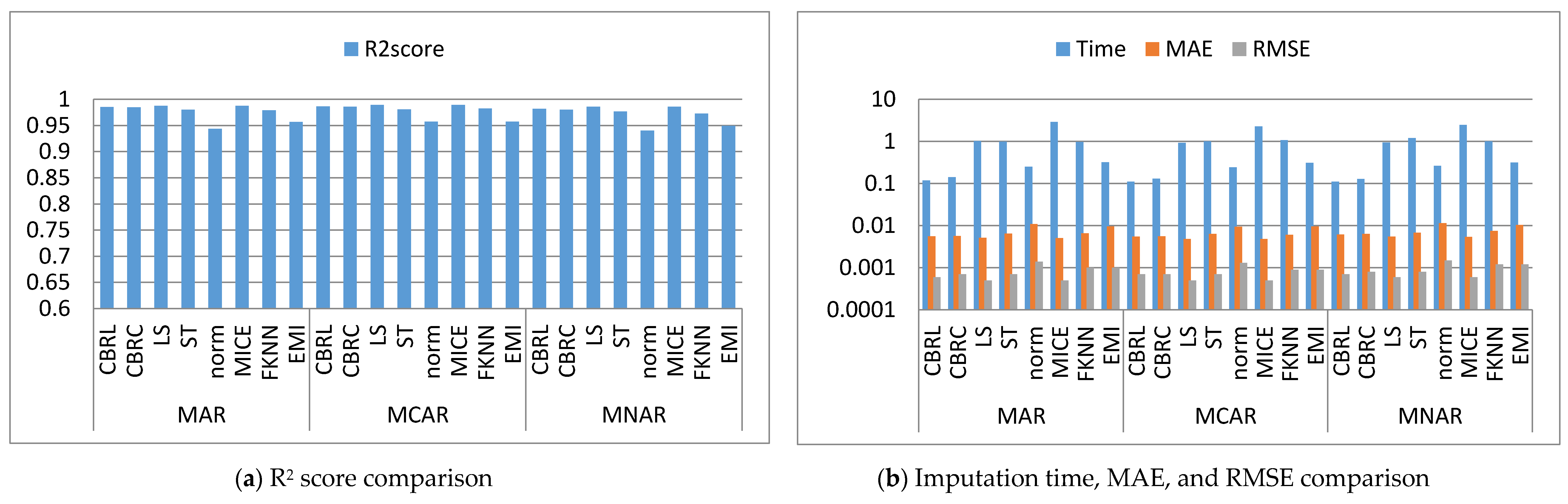
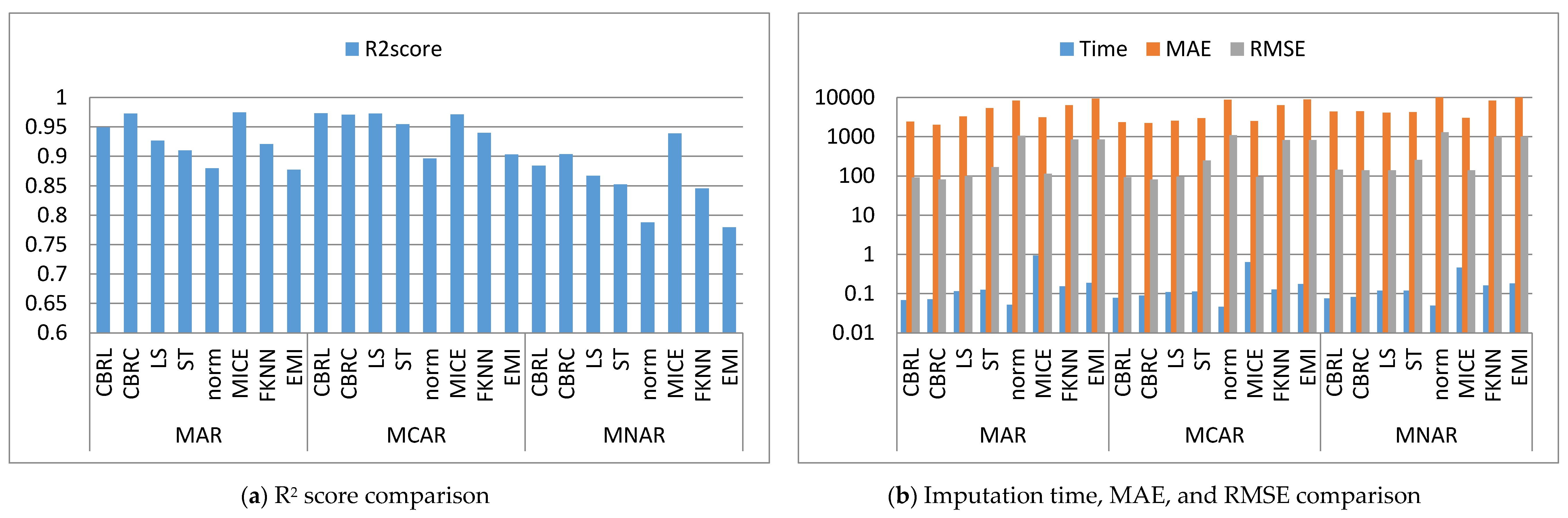
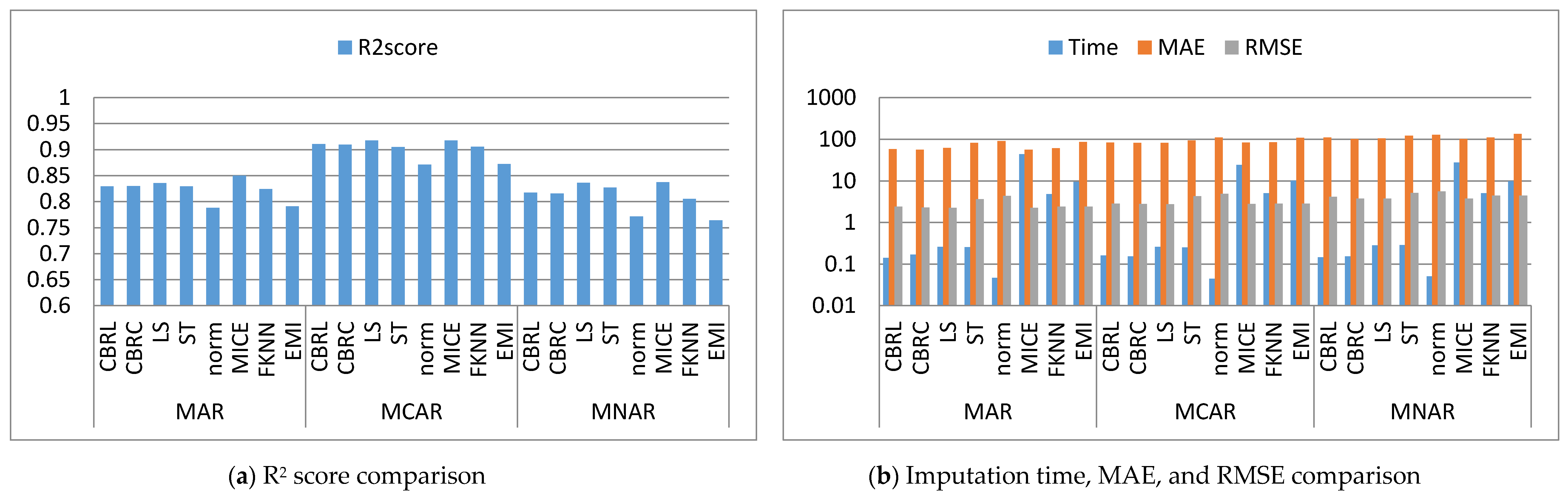
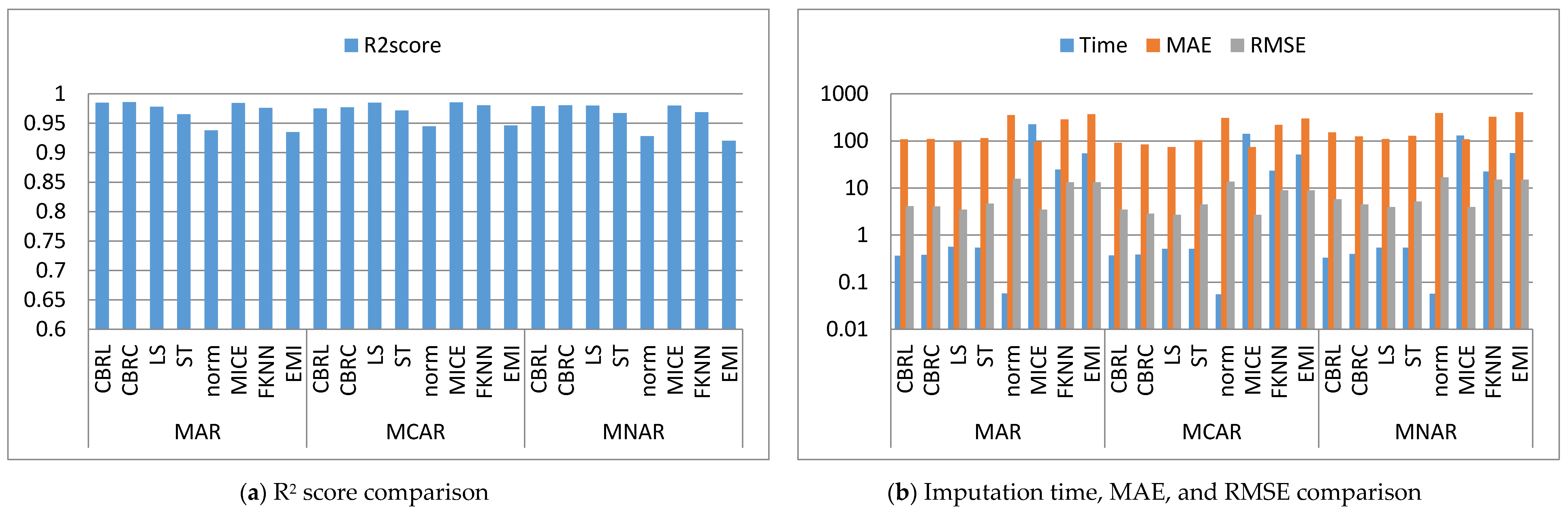
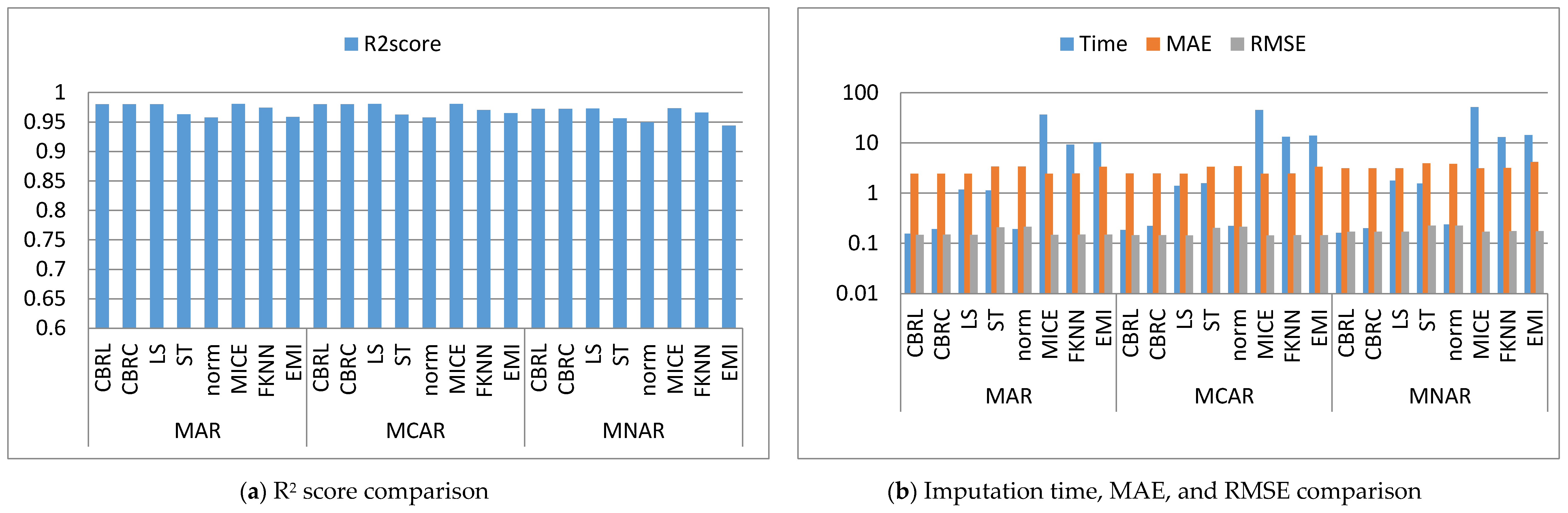
This subsection shows that CBRL and CBRC present lower errors in most cases. In what following, the error analysis is discussed in detail. Error analysis is represented by evaluating RMSE and MAE. It was remarked from Figure 2b and Figure 3b that the error produced by CBRL equals the error provided by least squares, and MICE. CBRC is worse than CBRL and better than stochastic, norm, Fast KNN, and EMI. From Figure 4b, it observed that CBRC is better in the provided error than other stated methods. Besides, CBRL equals in the provided error to least squares and MICE, and better than stochastic, norm, Fast KNN, and EMI. From Figure 5b, it was observed that CBRL and CBRC are worse than least squares and MICE in the provided error and better than stochastic, norm, Fast KNN, and EMI. CBRC is better than CBRL in MAR, worse in MCAR, and equals to each other in MNAR. In Figure 6b, it was observed that CBRL, CBRC, least squares, and MICE are equals in the provided error, and better than stochastic, norm, Fast KNN, and EMI. In Figure 7b, CBRL, and CBRC are worse than least squares and MICE and better than stochastic, norm, Fast KNN, and EMI in the provided error. CBRC is better than CBRL in the provided error. Figure 8b, Figure 9b, Figure 10b, Figure 11b, Figure 12b, Figure 13b, Figure 14b and Figure 15b, exhibit the error analysis for the BNG_heart_statlog and Poker Hand dataset using random samples of 10,000, 15,000, 20,000, and 50,000 of instances. As a result of taking samples from a dataset, the distribution becomes closer to Gaussian. Both CBRL and CBRC assume that independent features and the target feature have a normal distribution. So, CBRL and CBRC present lower errors on sample datasets. It is a better choice to apply transformers (e.g., Box-Cox and Yeo-Johnson) to the dataset before using any proposed algorithm. The error provided by CBRL, CBRC, least squares, and MICE is better than other stated methods. Also, CBRL is better than CBRC in the provided error.

4.2. Imputation Time

This subsection shows that CBRL and CBRC give better imputation time in most cases. In what following, the imputation time analysis is discussed in detail. Figure 2b and Figure 3b represent small size datasets it was remarked that CBRL and CBRC consume the lowest imputation time than other stated methods. Figure 4b, Figure 5b, Figure 6b and Figure 7b, show that CBRL and CBRC are faster in imputation time than least squares, MICE, Fast KNN, stochastic, and EMI and worse in imputation time than norm. For BNG_heart_statlog sample datasets, Figure 8b and Figure 9b show that CBRL and CBRC are faster than other stated methods. Figure 10b and Figure 11b show that CBRL and CBRC are better than other stated methods in imputation time but worse than norm. For Poker Hand sample datasets, Figure 12b shows that CBRL and CBRC are the fastest methods. In Figure 13b CBRL equals to norm, and better than other sated methods and CBRC is better than other stated methods and worth than norm. Figure 14b and Figure 15b show that CBRL and CBRC are better than all other stated methods but worse than norm.

4.3. Accuracy Analysis

This subsection shows that CBRL and CBRC give better accuracy in most cases. In what following, the accuracy analysis is discussed in detail. The accuracy indicates how the predicted values are close to the real data values. R² score (higher-value-is better). Figure 2a shows that CBRL equals to least squares and MICE in accuracy performance, and better than stochastic, norm, Fast KNN, and EMI. CBRC is worse in accuracy performance than CBRL, least squares, and MICE, and better than stochastic, norm, Fast KNN, and EMI. Figure 3a shows that CBRL is better in accuracy performance than stochastic, norm, Fast KNN and EMI, and worse than least squares and MICE. CBRC equals to CBRL in accuracy performance. Figure 4a CBRC is better in accuracy performance than all stated methods and worse than MICE. CBRL is better than all methods in accuracy performance and worth than CBRC and MICE. Figure 5a CBRL and CBRC are better in accuracy performance than stochastic, norm, Fast KNN, and EMI, but worse than least squares and MICE. CBRC is better in accuracy performance than CBRL. Figure 6a shows that CBRL and CBRC are better in accuracy performance than stochastic, norm, Fast KNN and EMI, and worse than least squares and MICE. CBRL is better in accuracy performance than CBRC. Figure 7a shows that in MAR, CBRL and CBRC are better in accuracy performance than least squares, stochastic, norm, Fast KNN and EMI, and equals to MICE. In MCAR, CBRL and CBRC are better in accuracy performance than stochastic, norm, Fast KNN, and EMI but worse than least squares and MICE. In MNAR, CBRL and CBRC are better in accuracy performance than stochastic, norm, Fast KNN and EMI, but equals to least squares and MICE. CBRC is better in accuracy performance than CBRL. Figure 8b, Figure 9b, Figure 10b, Figure 11b, Figure 12b, Figure 13b, Figure 14b and Figure 15b, exhibit the error analysis for the BNG_heart_statlog and Poker Hand dataset using random samples of 10,000, 15,000, 20,000, and 50,000 of instances. The results show that CBRL and CBRC equal in performance to least squares and MICE. CBRL and CBRC are better than stochastic, norm, Fast KNN, and EMI.

The results showed that CBRL, CBRC, least squares, and MICE present the lowest error and the highest accuracy. However, CBRL and CBRC are better than least squares and MICE in imputation time. CBRL is faster than CBRC. Least squares is faster than MICE. CBRC outperforms CBRL when data features are highly correlated as shown in Figure 4.

5. Conclusions

The quality of the data has a significant influence on the statistical analysis. Handling missing values in the dataset is a significant step in the data preprocessing stage. In conjunction with providing an impression of the studies associated with handling missing data, two imputation methods, CBRL and CBRC, based on feature selection conditions have been proposed in this paper to improve the quality of the data by utilizing from all available features. CBRL depends on selecting the feature with the smallest amount of missing data as the candidate feature. Choosing the feature with the smallest amount of missing data leads to building the model on the largest training data size, which in turn results in decreasing variance and the model is less prone to overfitting. CBRC works the same way as CBRL, except that it selects the feature with the highest correlation with the target feature. Although the correlation relationship between the independent features and the dependent feature is required, collinearity between input features is not required. The imputed feature will be used for imputing another incomplete feature until filling all missing values in all features. The proposed algorithms are easy to implement, work with any dataset at high speed, and do not fail in the imputation regardless of the size of the dataset, amount of missing data, or the missingness mechanism.

References

- Mostafa, S.M. Imputing missing values using cumulative linear regression. CAAI Trans. Intell. Technol. 2019, 4, 182–200. [Google Scholar] [CrossRef]
- Salgado, C.M.; Azevedo, C.; Manuel Proença, H.; Vieira, S.M. Missing data. Second. Anal. Electron. Health Rec. 2016, 143–162. [Google Scholar] [CrossRef] [Green Version]
- Hapfelmeier, A.; Hothorn, T.; Ulm, K.; Strobl, C. A new variable importance measure for random forests with missing data. Stat. Comput. 2014, 24, 21–34. [Google Scholar] [CrossRef] [Green Version]
- Batista, G.; Monard, M.-C. A study of k-nearest neighbour as an imputation method. Hybrid Intell. Syst. Ser. Front Artif. Intell. Appl. 2002, 87, 251–260. [Google Scholar]
- Aydilek, I.B.; Arslan, A. A hybrid method for imputation of missing values using optimized fuzzy c-means with support vector regression and a genetic algorithm. Inf. Sci. 2013, 233, 25–35. [Google Scholar] [CrossRef]
- Pampaka, M.; Hutcheson, G.; Williams, J. Handling missing data: Analysis of a challenging data set using multiple imputation. Int. J. Res. Method Educ. 2016, 39, 19–37. [Google Scholar] [CrossRef]
- Abdella, M.; Marwala, T. The use of genetic algorithms and neural networks to approximate missing data in database. Comput. Inform. 2005, 24, 577–589. [Google Scholar]
- Luengo, J.; García, S.; Herrera, F. On the choice of the best imputation methods for missing values considering three groups of classification methods. Knowl. Inf. Syst. 2012, 32, 77–108. [Google Scholar] [CrossRef]
- Donders, A.R.T.; van der Heijden, G.J.M.G.; Stijnen, T.; Moons, K.G.M. Review: A gentle introduction to imputation of missing values. J. Clin. Epidemiol. 2006, 59, 1087–1091. [Google Scholar] [CrossRef]
- Perkins, N.J.; Cole, S.R.; Harel, O.; Tchetgen Tchetgen, E.J.; Sun, B.; Mitchell, E.M.; Schisterman, E.F. Principled Approaches to Missing Data in Epidemiologic Studies. Am. J. Epidemiol. 2018, 187, 568–575. [Google Scholar] [CrossRef] [Green Version]
- Croiseau, P.; Génin, E.; Cordell, H.J. Dealing with missing data in family-based association studies: A multiple imputation approach. Hum. Hered. 2007, 63, 229–238. [Google Scholar] [CrossRef] [PubMed]
- Mostafa, S.M. Missing data imputation by the aid of features similarities. Int. J. Big Data Manag. 2020, 1, 81–103. [Google Scholar] [CrossRef]
- Iltache, S.; Comparot, C.; Mohammed, M.S.; Charrel, P.J. Using semantic perimeters with ontologies to evaluate the semantic similarity of scientific papers. Informatica 2018, 42, 375–399. [Google Scholar] [CrossRef] [Green Version]
- Yadav, M.L.; Roychoudhury, B. Handling missing values: A study of popular imputation packages in R. Knowl.-Based Syst. 2018, 160, 104–118. [Google Scholar] [CrossRef]
- Farhangfar, A.; Kurgan, L.A.; Pedrycz, W. A Novel Framework for Imputation of Missing Values in Databases. IEEE Trans. Syst. Man Cybern. Part A Syst. Hum. 2007, 37, 692–709. [Google Scholar] [CrossRef]
- Zahin, S.A.; Ahmed, C.F.; Alam, T. An effective method for classification with missing values. Appl. Intell. 2018, 48, 3209–3230. [Google Scholar] [CrossRef]
- Batista, G.E.A.P.A.; Monard, M.C. An analysis of four missing data treatment methods for supervised learning. Appl. Artif. Intell. 2003, 17, 519–533. [Google Scholar] [CrossRef]
- Acuña, E.; Rodriguez, C. The Treatment of Missing Values and its Effect on Classifier Accuracy. In Classification, Clustering, and Data Mining Applications; Springer: Berlin/Heidelberg, Germany, 2004; pp. 639–647. [Google Scholar]
- Li, D.; Deogun, J.; Spaulding, W.; Shuart, B. Towards Missing Data Imputation: A Study of Fuzzy K-means Clustering Method. In Proceedings of the International Conference on Rough Sets and Current Trends in Computing, Madrid, Spain, 9–13 July 2004; Springer: Berlin/Heidelberg, Germany, 2004; Volume 3066, pp. 573–579. [Google Scholar]
- Feng, H.; Chen, G.; Yin, C.; Yang, B.; Chen, Y. A SVM regression based approach to filling in missing values. In Proceedings of the International Conference on Knowledge-Based and Intelligent Information and Engineering Systems, Melbourne, Australia, 14–16 September 2005; Springer: Berlin/Heidelberg, Germany, 2005; Volume 3683, pp. 581–587. [Google Scholar] [CrossRef]
- Choudhury, S.J.; Pal, N.R. Imputation of missing data with neural networks for classification. Knowl.-Based Syst. 2019, 182. [Google Scholar] [CrossRef]
- Muñoz, J.F.; Rueda, M. New imputation methods for missing data using quantiles. J. Comput. Appl. Math. 2009, 232, 305–317. [Google Scholar] [CrossRef]
- Twala, B.; Jones, M.C.; Hand, D.J. Good methods for coping with missing data in decision trees. Pattern Recognit. Lett. 2008, 29, 950–956. [Google Scholar] [CrossRef] [Green Version]
- Varoquaux, G.; Buitinck, L.; Louppe, G.; Grisel, O.; Pedregosa, F.; Mueller, A. Scikit-learn. J. Mach. Learn. Res. 2011, 12, 2825–2830. [Google Scholar] [CrossRef]
- Chandrashekar, G.; Sahin, F. A survey on feature selection methods. Comput. Electr. Eng. 2014, 40, 16–28. [Google Scholar] [CrossRef]
- Van Buuren, S.; Groothuis-Oudshoorn, K.; Robitzsch, A.; Vink, G.; Doove, L.; Jolani, S.; Schouten, R.; Gaffert, P.; Meinfelder, F.; Gray, B. MICE: Multivariate Imputation by Chained Equations. 2019. Available online: https://cran.rproject.org/web/packages/mice/ (accessed on 15 March 2019).
- Efron, B.; Hastie, T.; Iain, J.; Robert, T. Diabetes Data. 2004. Available online: https://www4.stat.ncsu.edu/~boos/var.select/diabetes.html (accessed on 1 June 2019).
- Acharya, M.S. Graduate Admissions-1-6-2019. Available online: https://www.kaggle.com/mohansacharya/graduate-admissions (accessed on 1 June 2019).
- Stephen, B. Profit Estimation of Companies. Available online: https://github.com/boosuro/profit_estimation_of_companies (accessed on 8 August 2019).
- Kartik, P. Red & White Wine Dataset. Available online: https://www.kaggle.com/numberswithkartik/red-white-wine-dataset (accessed on 11 February 2019).
- Cam, N. California Housing Prices. Available online: https://www.kaggle.com/camnugent/california-housing-prices (accessed on 6 July 2019).
- Magrawal, S. Diamonds. Available online: https://www.kaggle.com/shivam2503/diamonds (accessed on 30 August 2019).
- Cattral, R.; Oppacher, F. Poker Hand Dataset. Available online: https://archive.ics.uci.edu/ml/datasets/Poker+Hand (accessed on 24 November 2019).
- Holmes, G.; Pfahringer, B.; van Rijn, J.; Vanschoren, J. BNG_heart_statlog. Available online: https://www.openml.org/d/267 (accessed on 11 September 2019).
- Kearney, J.; Barkat, S. Autoimpute. Available online: https://autoimpute.readthedocs.io/en/latest/ (accessed on 1 January 2020).
- Law, E. Impyute. Available online: https://impyute.readthedocs.io/en/latest/ (accessed on 8 August 2019).
- Chai, T.; Draxler, R.R. Root mean square error (RMSE) or mean absolute error (MAE)? -Arguments against avoiding RMSE in the literature. Geosci. Model Dev. 2014, 7, 1247–1250. [Google Scholar] [CrossRef] [Green Version]