
Abstract
Discrete element modeling (DEM) of polydisperse granular materials is significantly more computationally expensive than modeling of monodisperse materials as a larger number of particles are required to obtain a representative elementary volume, and standard contact detection algorithms become progressively less efficient with polydispersity. This paper presents modified contact detection and inter-processor communication schemes implemented in LAMMPS which account for particles of different sizes separately, greatly improving efficiency. This new scheme is applied to the inertial number (I), which quantifies the ratio of inertial to confining forces. This has been used to identify the quasi-static limit for shearing of granular materials, which is often taken to be \( I = 10^{ - 3} \). However, the expression for the inertial number contains a particle diameter term and therefore it is unclear how to apply this for polydisperse media. Results of DEM shearing tests on polydisperse granular media are presented in order to determine whether \( I \) provides a unique quasi-static limit regardless of polydispersity and which particle diameter term should be used to calculate \( I \). The results show that the commonly used value of \( I = 10^{ - 3} \) can successfully locate the quasi-static limit for monodisperse media but not for polydisperse media, for which significant variations of macroscopic stress ratio and microscopic force and contact networks are apparent down to at least \( I = 10^{ - 6} \). The quasi-static limit could not be conclusively determined for the polydisperse samples. Based on these results, the quasi-staticity of polydisperse samples should not be inferred from a low inertial number as currently formulated, irrespective of the particle diameter used in its calculation.
1 Introduction
Polydisperse granular materials (i.e., those containing a range of particle sizes) occur in many physical and industrial settings, such as geomaterials, avalanches and landslides, crushing of mining ores and food processing. Often the range of particle sizes in such systems covers several orders of magnitude. For example, the granular filter material used to construct the Bennett Dam in Canada contains particles ranging from 0.08 to 75 mm [1]. Such a range of length scales presents significant computation challenges to the discrete element method (DEM), typically used to model such systems. These challenges reflect the fact that in polydisperse systems (i) a larger number of particles are required to obtain a representative elementary volume (REV) than for a monodisperse system and (ii) the standard contact detection algorithms used in such modeling can become progressively less effective with increasing particle size ratio.
While growing computational power has allowed effective investigation of increasingly polydisperse systems [2,3,4], and algorithmic enhancements in contact detection [5, 6] have improved the efficiency of such simulations, there remain challenges. This remains particularly true for simulations requiring long timescales. Many physical processes and standard laboratory tests such as geomechanical element testing involve extremely low strain rates imposed over a long time period, and it can generally be assumed that quasi-static shearing occurs. These conditions would be impractical to replicate in a DEM simulation of reasonable computational cost, so the simulated strain rates are artificially increased by orders of magnitude. Correspondence between the simulations and reality is maintained by loading the granular material quasi-statically, i.e., the loading occurs sufficiently slowly that inertial effects can be neglected. In order to identify the boundary between the quasi-static and inertial or dense-flow regimes, the dimensionless inertial number \( I = \dot{\varepsilon }d\sqrt {\frac{\rho }{p}} \) is used, where \( \dot{\varepsilon } \) is the shear rate, d is particle diameter, \( \rho \) is particle density and \( p \) is the mean confining stress [2, 3]. The inertial number represents the ratio of inertial to confining forces, and as \( I \to 0 \), the flow regime tends to the quasi-static limit. Radjai [4] states that “For a confining pressure \( p \) (counted positive for compressive stresses) and particles of average diameter \( d \), the contact forces of static origin are of the order of \( f_{\rm s} = pd^{2} \)… At the same time, for a shear strain rate \( \dot{\epsilon }_{q} \), the timescale of the flow is \( \mathop {\Delta t = \dot{\epsilon } }\limits_{q}^{ - 1} \) and thus the order of magnitude of the impulsive forces is given by the momentum per unit time \( f_{i} = md\dot{\epsilon }_{q} /\Delta t \), where \( m \) is the average particle mass. In the quasi-static limit, the condition \( f_{\rm s} \gg f_{i} \) implies \( I \equiv \dot{\epsilon }_{q} \sqrt {\frac{m}{pd}} \ll 1 \).” Andreotti et al. [5] explain that \( I \) can be interpreted as the ratio between two timescales: \( I = \frac{{t_{\text{micro}} }}{{t_{\text{macro}} }} \), where \( t_{\text{micro}} = \frac{d}{{\sqrt {p/\rho_{d} } }} \), representing the rate of microscopic rearrangements of particles subject to a pressure \( p \), and \( t_{\text{macro}} = \frac{1}{{\dot{\varepsilon }}} \), representing the macroscopic shear rate. In the quasi-static regime, macroscopic rearrangements can be considered to occur very slowly in comparison with the microscopic rearrangements.
Based on the empirical assessment of 2D DEM simulation results of plane shear tests, da Cruz et al. [2] set the practical limit of the quasi-static regime at \( I \le 10^{ - 3} \). Considering conditions at the critical state in 3D DEM simulations of geotechnical element testing, Perez et al. [3, 6] found the limit at \( I \le 7.9 \times 10^{ - 5} \).
The above work has been influential in improving the quality of DEM simulations for granular materials under quasi-static conditions in that it is now relatively common to set shear rates so that \( I \le 10^{ - 3} \) or \( I \le 10^{ - 4} \). However, the use of a single particle diameter, \( d \), in the calculation of \( I \) suggests a monodisperse material. In reality, many granular materials, including most geomaterials, are polydisperse. An ideal definition of inertial number would be able to identify a unique quasi-static limit regardless of the particle size distribution of the material under shear. The selection of an appropriate diameter term for use in the calculation of inertial number is required to define such an inertial number. Apart from the work of Rognon et al. [7], who proposed a packing fraction-weighted inertial number to account for granular flows involving disks of a different diameter to account for segregation, there has been very little work to examine the effectiveness of inertial number in defining the quasi-static limit for polydisperse materials.
To provide access to the low strain rates and long timescales required to address the question of where the effective inertial regime lies in polydisperse systems, this paper first addresses an improved contact detection method implemented in the popular molecular dynamics code LAMMPS [8]. A series of DEM triaxial compression tests is then carried out at varying shear rates on materials with varying degrees of polydispersity using the new contact detection method. Analysis of a selection of preliminary results allows the validity of the previously proposed limits for quasi-static behavior to be examined using various diameter terms to calculate the inertial number.
2 Methodology
2.1 Modified DEM model
DEM simulations were carried out using a modified version of the open-source DEM code Granular LAMMPS [8]. In order to improve efficiency when simulating highly polydisperse materials, the contact detection and inter-processor communication algorithms in LAMMPS were modified from the existing link-cell method [8] to a new method termed the hierarchical stencil method, which is conceptually similar to the hierarchical grid Method used in MercuryDPM [9, 10] but utilizes the existing LAMMPS stencil capabilities developed by in’t Veld et al. [11]. A brief outline of the modification is given here; full details of the implementation and parametric studies are available at [12].
The existing LAMMPS contact detection is a combination of the widely used Verlet neighbor list and link-cell methods [8]. In DEM simulations, Verlet neighbor lists store all pairs of particles which are within a distance 2rskin of each other, where rskin is the “skin distance,” as defined in Fig. 1. The additional skin distance means the neighbor list must be constructed intermittently (e.g., when any particle has moved a distance of rskin/2 since the last rebuild). At each intermediate timestep, only the particle pairs on the neighbor list are checked for contact; where contact exists, the force is calculated. To avoid brute-force construction of the neighbor list, the link-cell method is used. A regular grid of cells is overlaid on the DEM domain, and, for each particle, a subset of link cells are searched to create the neighbor list. For example, in Fig. 1 the link-cell length is \( r_{\text{cell}} = r_{ \rm{max} } + r_{\text{skin}} \). Considering the green particle in Fig. 1, the neighbor list is constructed by checking the “home” link cell plus surrounding link cells within 2 \( r_{\rm c} \). The list of cells to be checked is stored in a pre-computed stencil [11].

Schematic showing link-cell contact detection in LAMMPS, where rmax is the maximum particle radius, and rc is the cell dimension. rc = rmax + rskin where rskin is the skin distance
LAMMPS implements a standard approach of domain decomposition with message passing via the message passing interface (MPI) in parallel. This means that particles are “owned” by a given MPI task dependent on their position. In order that all relevant interactions may be located, a given local domain must obtain information on particles in adjoining regions. Communication of ghost particles within a “halo” of cells with dimension \( r_{\text{halo}} = 2r_{\rm c} \) is performed to fulfill this requirement, as shown in Fig. 2.

2D schematic of inter-processor communication in LAMMPS. Particle information within the halo of dimension rhalo must be communicated to the processor subdomain at every timestep
The Verlet/link-cell method is highly efficient for monodisperse packings of particles. However, as the packings considered become increasingly polydisperse, the efficiency of the method reduces [12]. Consider a granular system with two types of particle having radii \( r_{\rm s} \) and \( r_{\rm l} \) (for small and large). This introduces three different interaction cutoff ranges: \( r_{\rm c}^{\rm ss} \), \( r_{\rm c}^{\rm sl} \) and \( r_{\rm c}^{\rm ll} \). In principle, one should choose the cell width to be \( r_{\rm cell} \) = \( 2r_{\rm c}^{\rm ll} \) to ensure all large–large interactions are captured. However, the resulting cell size will necessarily drag into the search very many small–large and small–small pairs well beyond their respective cutoffs. This is inefficient and becomes more inefficient as the ratio \( r_{\rm l} \)/\( r_{\rm s} \) increases. Similarly, the communication halo will be of dimension \( r_{\rm halo} \) = \( 2r_{\rm c}^{\rm ll} \). Therefore, as the link-cell and halo sizes are both based on the largest particle, for polydisperse packings many more particle pairs must be considered in neighbor list construction and inter-processor communication than for monodisperse packings.
The new hierarchical stencil method overcomes this limitation as follows:
-
Particle types are allocated based on particle radius;
-
Cell lists are instantiated for each particle type. The sizes of the link cells are based on the largest particle of each type in a similar way to Ogarko and Luding [9]. For example, for a bidisperse system, two particle types and two cell lists with sizes \( r_{\rm c}^{s} \) and \( r_{\rm c}^{\rm l} \) are instantiated.
-
Interactions between particles of the same type are identified using a stencil within the appropriate cell list as shown schematically in Fig. 3 for a bidisperse system.
Fig. 3 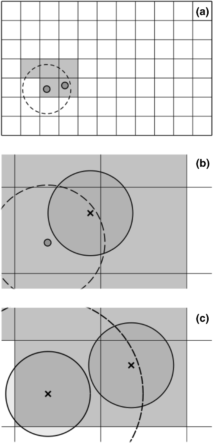
2D schematic showing interactions between different particle types: a small–small interactions; b small–large interactions; c large–large interactions
-
For interactions between two particles of different types, particle i is located within the cell list of the j-type particles. An appropriate stencil is then used to perform the neighbor list construction in the j-type cell list. The most efficient way to locate particles is using a one-way search which identifies potential small–large pairs by considering only small particles and using the large particle cell list to search for interactions, and using a symmetric stencil in the large cell list (Fig. 3b) to examine large neighbors [12].
-
In’t Veld et al. [11] improved the existing LAMMPS inter-processor communication by introducing multiple halos for different interaction types. For a bidisperse system, the halo width is \( r_{\rm halo}^{\rm sl} \) for small particles and \( r_{\rm halo}^{\rm ll} \) for large particles, where, for example, \( r_{\rm halo}^{\rm sl} = r_{\rm c}^{s} + r_{\rm c}^{\rm l} \) as shown in Fig. 4. This is sufficient to allow identification of all potential pairs. Potential small–small pairs may be located on the basis of \( r_{\rm halo}^{\rm ss} \). In addition, a significant efficiency saving can be made as all potential small–large pairs are located by examining owned small particles, meaning no small ghost particles beyond \( r_{\rm c}^{\rm ss} \) are required. The ghost cutoff distance for large particles is unchanged at \( r_{\rm halo}^{\rm ll} \), and potential large–large pairs are identified as before.
Fig. 4 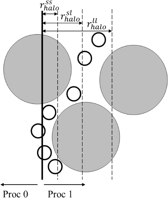
Schematic of hierarchical stencil inter-processor communication (adapted from [11]). Halos of different dimensions are adopted depending on the interaction type (i.e., large–large, small–large or small–small)
-
The discussion thus far has focused on bidisperse systems. Generalization of the scheme to polydisperse systems is straightforward. A number of cell lists of varying size are selected, and particle i is assigned a type based on the smallest cell for which \( r_{i} + r_{\rm skin} \le r_{\rm c} \). The number and size of cell lists must then be selected. Previous studies [13] suggest this is strongly dependent on the particle size distribution for the problem at hand, and no general law is available to decide without testing. However, for the continuous polydisperse systems simulated here it was found that two or three cell lists with a logarithmic size spacing were optimal [12]. This is in contrast to the findings of Krijgsman et al. [13] for the hierarchical grid method, highlighting that although the two schemes are conceptually similar, important differences in implementation exist.


More detail on the classes of the C ++ implementation in LAMMPS is given in [12]. The implementation was validated using the analytical solution developed for the failure stress ratios in a face-centered cubic assembly of uniform rigid spheres [14] in which multiple particle types were assigned. A further validation was carried out by comparing the results of triaxial compression simulations using 74,504 particles to the existing link-cell contact detection schemes. The variation in coordination number and stress ratio at the critical state were found to be a fraction of a percent, representing rounding errors accumulated due to the neighbor lists being assessed in a different order with the different schemes.
The speedup of the hierarchical stencil method over the link-cell method improves with increasing size ratio. For size ratios of \( r_{\rm max} /r_{min} \) = 10, speedups were at least 10, and for \( r_{\rm max} /r_{min} \) = 100, speedups of up to 400 versus the existing link-cell method without communication improvements were obtained [12]. The hierarchical stencil also scales well to at least 768 processors, with scaling being greatly improved by the inter-processor communication improvements [12].
2.2 DEM simulations
A total of 76 DEM simulations of constant mean stress triaxial tests were carried out. Seven different polydisperse particle size distributions (PSDs) were simulated, as shown in Fig. 5. Samples of series “A” have an equal volume of particles per log diameter bin, whereas samples of series “B” have an equal volume of particles per linear diameter bin. Series A therefore have relatively more fine particles. The number of particles in each sample is presented in Table 1. These were selected on a trial-and-error basis, taking care to ensure that an REV was achieved for each sample so that the sample responses with respect to I are meaningful. Unfortunately, no clear relationship can be established between grading and number of particles for an REV. A conservative timestep of \( 7.5 \times 10^{ - 8} \) s was used in all simulations, calculated using \( \Delta t = 0.1 \sqrt {\frac{{m_{\rm{min} } }}{{K_{\rm{max} } }}} \) where \( m_{min} \) is the minimum particle mass and \( K_{max} \) is the maximum contact stiffness [15] calculated using a 2% particle overlap (actual overlaps in the simulations at no point exceeded 1%).

Particle size distributions
In each test, the particles were initially generated in a random, non-touching cloud, before being isotropically compressed to \( p^{\prime} = 100\,{\text{kPa}} \). A simplified Hertz–Mindlin contact model was used with shear modulus G = 29 GPa and Poisson’s ratio ν = 0.2. The initial interparticle friction coefficient of μ = 0.15 was used during compression to create an initially dense packing configuration. Following isotropic compression, the friction was set to μ = 0.3 and the sample allowed to equilibrate. During shearing, the mean normal stress was maintained at \( p^{\prime} = 100\,{\text{kPa}} \) to allow a constant value of I to be maintained [3]. For each PSD, a series of tests were carried out in which the axial shear rate, \( \dot{\varepsilon }_{1} \), was varied to impose different values of inertial number calculated using the maximum particle diameter, \( I_{\text{dmax}} = \dot{\varepsilon }_{1} d_{ \rm{max} } \sqrt {\frac{\rho }{p}} \), ranging from \( I_{d{\rm max}} = 5 \times 10^{ - 3} \) to \( I_{d{\rm max}} = 5 \times 10^{ - 6} \) for samples with χ = dmax/dmin = 1.2 to 5 and \( I_{d{\rm max}} = 5 \times 10^{ - 3} \) to \( I_{d{\rm max}} = 1 \times 10^{ - 6} \) for samples with χ = 10 and 20. \( I_{d{\rm max}} \) was selected as the default inertial number as it gives the largest value of I. \( I_{d{\rm max}} = 1 \times 10^{ - 6} \) was proved to be the slowest simulation which could be practically carried out: To shear to \( \varepsilon_{1} = 2\% \) at this rate, sample A20 required around 480 h using 180 cores and B20 required 288 h using 72 cores on the Cirrus HPC facility (http://www.cirrus.ac.uk/). To reduce \( I_{d{\rm max}} \) by a further order of magnitude would have been computationally infeasible.
3 Results and discussion
Plots of axial strain against stress ratio \( \eta = \frac{q}{p} \), where q is the deviatoric stress, volumetric strain \( \varepsilon_{\rm v} \) and mechanical coordination number \( Z_{\rm mech} \) (the average number of contacts per stress-transmitting particle) for simulations with \( I_{d{\rm max}} = 1 \times 10^{ - 3} \) are shown in Figs. 6, 7 and 8. These strains are sufficient to allow the effect of I on material behavior to be determined in what Roux [16] called Regime 2, in which particle rearrangements control the macroscale quasi-static response. At this fixed inertial number, \( \eta \) and \( |\varepsilon_{\rm v} | \) increase, while \( Z_{\rm mech} \) decreases with increasing χ.

Stress ratio behavior during shearing at \( I_{d{\rm max}} = 1 \times 10^{ - 3} \)

Volumetric behavior during shearing at \( I_{d{\rm max}} = 1 \times 10^{ - 3} \)

Mechanical coordination number during shearing at \( I_{d{\rm max}} = 1 \times 10^{ - 3} \)
3.1 Variation of sample response with I dmax
Figure 9 shows the stress ratio at \( \varepsilon_{1} = 2\% \) with varying \( I_{d{\rm max}} \) for all samples. The stress ratios are normalized by their values at \( I_{d{\rm max}} = 1 \times 10^{ - 3} \), which are shown in Fig. 6. The most uniform sample, A1.2, shows approximately constant values at \( I_{d{\rm max}} \le 1 \times 10^{ - 3} \). For all other samples, the stress ratio reduces with inertial number with no sign of a plateau in values at \( I_{d{\rm max}} = 1 \times 10^{ - 6} \), most significantly for sample B20 for which \( \eta = 0.846 \eta_{{\left( {1e - 3} \right)}} \). Interestingly, the trends do not exactly follow χ; most notably, A10 shows more variation with \( I_{d{\rm max}} \) than A20. Figure 10 shows normalized values of solid packing fraction ϕ at \( \varepsilon_{1} = 2\% \). Apart from the near-monodisperse A1.2, all samples show an increase in packing fraction as the inertial number reduces, although the magnitude of this change is less significant than for the stress ratio. In contrast, mechanical coordination number (Fig. 11) shows a similar trend regardless of the particle size distribution, with a small increase in normalized values as inertial number reduces.

Effect of \( I_{d{\rm max}} \) on stress ratio at \( \varepsilon_{1} = 2\% \). Results are normalized by the response at \( I_{d{\rm max}} = 1 \times 10^{ - 3} \): a series A; b series B

Effect of \( I_{d{\rm max}} \) on solid packing fraction at \( \varepsilon_{1} = 2\% \). Results are normalized by the response at \( I_{d{\rm max}} = 1 \times 10^{ - 3} \): a series A; b series B

Effect of \( I_{d{\rm max}} \) on mechanical coordination number at \( \varepsilon_{1} = 2\% \). Results are normalized by the response at \( I_{d{\rm max}} = 1 \times 10^{ - 3} \): a series A; b series B
Further insight into changes in the stress-transmitting fabric of the sample showing the greatest variation in \( \eta \) with \( I_{d{\rm max}} \), B20, is given in Figs. 12a, b and 13a, which, respectively, show the probability density functions of normal contact force and the relative frequency distribution of connectivity (number of stress-transmitting contacts per particle). In Fig. 12a, b it can be seen that the force network tends to become more inhomogeneous as the inertial number increases (resembling the increasing force inhomogeneity found by Voivret et al. [17] in 2D and Mutabaruka et al. [18] in 3D with increasing polydispersity). This suggests that at higher inertial numbers the deviatoric stress-transmitting strong-force network is more dominant, which explains the higher stress ratios at higher inertial numbers. Despite the relatively small changes in mechanical coordination number (Fig. 11), the number of contacts per particle shows significant differences between samples sheared with different inertial numbers (Fig. 13a). The more slowly a sample is sheared, the fewer relatively unstable particles with C = 2 or 3 or highly connected particles with C ≥ 18 are present. However, there are more particles with 4 ≤ C ≤ 17 when inertial numbers are low. In contrast, the near-monodisperse sample A1.2 has almost indistinguishable force and contact distributions for all samples with \( I_{d{\rm max}} \le 1 \times 10^{ - 3} \) as shown in Figs. 12c and 13b. Considering both macro- and microscale results, it can be concluded that a true quasi-static limit has not been reached for the polydisperse samples with \( \chi \ge 5 \). For frictional particles, the minimum number of contacts for static mechanical stability is 4 [19], and therefore, the number of particles with four or more contacts can be taken as a measure of quasi-staticity [3, 20]. This was termed the non-rattler fraction fNR by Bi et al. [21] and is plotted against inertial number normalized by values at \( I_{d{\rm max}} = 10^{ - 3} \) in Fig. 14a and as raw values in Fig. 14b. Two features to note are: (i) More polydisperse samples have a much lower fNR (i.e., a greater proportion of rattlers) and (ii) fNR reduces with \( I_{d{\rm max}} \) for the more polydisperse samples. Shen and Sankaran [22] demonstrated that at higher strain rates the coordination number reduces, but the size of groups of interconnected particles (analogous to the non-rattlers) increases, similar to the trend seen here. Large numbers of rattlers will naturally be present in all highly polydisperse materials. It is possible that at inertial numbers around the previously defined quasi-static (monodisperse) limit (\( I = 10^{ - 3} ) \) these rattlers are more able to join and stabilize buckling force chains [23, 24] than at either higher or lower inertial numbers. This would account for the higher stress ratio and packing fraction at inertial numbers close to the monodisperse limit. These rattlers would be the smaller particles, which would be “captured” by the larger particles upon force chain buckling [25]. Interestingly, at \( I_{d{\rm max}} = 5 \times 10^{ - 3} \) (above the usual definition for the quasi-static limit) the non-rattler fraction and stress ratio are both higher, suggesting that this rattler “capturing” mechanism is mainly found below the monodisperse quasi-static limit. However, the relationship between rattlers and quasi-staticity requires further study.

Probability density functions of normal contact force, N, normalized by mean normal contact force, < N >. a Sample B20; b sample A1.2

Relative frequency plot of connectivity, C: a sample B20, contacts C ≤ 6 (note linear y-scale); b sample B20, contacts C ≥ 6 (note log y-scale); c sample A1.2, contacts C ≤ 6

Effect of \( I_{d{\rm max}} \) on non-rattler fraction fNR at \( \varepsilon_{1} = 2\% \): a series A; b series B
3.2 Alternative definitions of inertial number
Figure 15 presents the variation of normalized stress ratio for the series B tests with inertial number where two alternative definitions of inertial number are used: (i) \( I_{d50} = \dot{\varepsilon }_{1} d_{50} \sqrt {\frac{\rho }{p}} \), where \( d_{50} \) is the median particle diameter (for which 50% of particles by volume are smaller) and (ii) \( I_{{{\bar{\text{d}}}}} = \dot{\varepsilon }_{1} \bar{d}\sqrt {\frac{\rho }{p}} \), where \( \bar{d} = \frac{{\mathop \sum \nolimits_{i = 1}^{{N_{\rm mech} }} \left( {d_{i} V_{p,i} } \right)}}{{\mathop \sum \nolimits_{i = 1}^{{N_{\rm mech} }} V_{p,i} }} \), \( N_{\rm mech} \) is the number of particles with two or more contacts, \( d_{i} \) is the diameter of particle i and \( V_{p,i} \) is the volume of particle i. \( I_{{{\bar{\text{d}}}}} \) takes a form similar to that proposed by Rognon et al. [7] for bidisperse granular flows. For both \( I_{d50} \) and \( I_{{{\bar{\text{d}}}}} \), there is a similar trend of reducing \( \eta \) with inertial number, but the minimum inertial numbers are lower for \( I_{d50} \) and \( I_{{{\bar{\text{d}}}}} \) than for \( I_{d{\rm max}} \).

Effect of alternative inertial number definitions on stress ratio at \( \varepsilon_{1} = 2\% \): a \( I_{d50} \); b \( I_{{{\bar{\text{d}}}}} \)
As the quasi-static limit has not been reached for samples with \( \chi \ge 5 \), the most effective inertial number for determining this limit cannot be established. As explained in the Introduction, the fundamental concept of inertial number is a ratio between the impulsive forces and the contact forces of static origin [4]. For a polydisperse granular material, the largest possible inertial number, as currently defined, requires maximizing the order of magnitude of the impulsive forces by using the largest particle diameter and mass in its calculation, while minimizing the contact forces of static origin by using the smallest particle diameter. In that “worst possible” case, the inertial number would be \( \chi I_{d{\rm max}} \). Therefore, the current definition of inertial number does not permit differences in inertial number of more than three orders of magnitude compared to the uniform case, irrespective of the definition of particle diameter adopted. Hence, the inertial number, as currently defined, is not appropriate for locating the quasi-static limit for polydisperse granular materials.
4 Conclusions
Particulate simulations of continuously polydisperse granular materials with χ = dmax/dmin = 1.2 to 20 were carried out using a DEM code which was modified for increased efficiency with polydisperse media. This was achieved by introducing a hierarchy of cell lists and improved inter-processor communication for particles of a different diameter. In order to investigate whether the quasi-static limit is the same for granular materials regardless of their particle size distribution, the polydisperse samples were sheared under triaxial compression to \( \varepsilon_{1} = 2\% \) with inertial numbers calculated using the maximum particle diameter ranging from \( I_{d{\rm max}} = 5 \times 10^{ - 3} \) to \( I_{d{\rm max}} = 1 \times 10^{ - 6} \). From the results, the following conclusions can be drawn:
-
For a near-monodisperse particle size distribution (χ = 1.2), the quasi-static limit was found at approximately \( I_{\text{dmax}} \le 1 \times 10^{ - 3} \), in agreement with previous studies [2].
-
For the more polydisperse distributions, the quasi-static limit was not found even at \( I_{d{\rm max}} = 1 \times 10^{ - 6} \) and, in general, more polydisperse distributions showed a greater reduction in stress ratio and more homogeneous force and contact networks with a reduction in inertial number.
-
More polydisperse distributions have more rattlers, and the proportion of rattlers increases as inertial number reduces below \( I_{d{\rm max}} = 1 \times 10^{ - 3} \). These rattlers may be less likely to join and stabilize force chains at low inertial numbers, leading to a lower stress ratio.
-
Definitions of inertial number using alternative diameter definitions, for example the median particle diameter, \( I_{d50} \), or a volume-weighted diameter, \( I_{{\bar{d}}} \), are also unable to determine a unique quasi-static limit regardless of particle size distribution.
As currently defined, the inertial number is not appropriate for locating the quasi-static limit for polydisperse granular materials. Further work is required to determine where the quasi-static limit lies for polydisperse media and to establish whether the inertial number could be somehow adapted to find this limit accounting for polydispersity. As both computational resources increase in power and further algorithmic improvements can be identified, it is hoped that future work will be able to access more highly polydisperse systems at yet smaller inertial numbers. Such simulations should be able to identify more exactly where the limiting inertial number lies.
References
Wood DM (2007) The magic of sands—the 20th Bjerrum Lecture presented in Oslo, 25 November 2005 1. Can Geotech J 20th Bjerr:1329–1350
Da Cruz F, Emam S, Prochnow M et al (2005) Rheophysics of dense granular materials: discrete simulation of plane shear flows. Phys Rev E Stat Nonlinear Soft Matter Phys. https://doi.org/10.1103/PhysRevE.72.021309
Lopera Perez JC, Kwok CY, O’Sullivan C et al (2016) Assessing the quasi-static conditions for shearing in granular media within the critical state soil mechanics framework. Soils Found. https://doi.org/10.1016/j.sandf.2016.01.013
Radjai F (2009) Force and fabric states in granular media. In: AIP conference proceedings
Andreotti B, Forterre T, Pouliquen O (2013) Granular media: between fluid and solid. Cambridge University Press, Oxford
Lopera Perez JC, Kwok CY, O’Sullivan C et al (2017) Erratum to “Assessing the quasi-static conditions for shearing in granular media within the critical state soil mechanics framework” (Soils and Foundations (2016) 56(1) (152–159) (S0038080616000147) (10.1016/j.sandf.2016.01.013)). Soils Found
Rognon PG, Roux J-N, Naaïm M, Chevoir F (2007) Dense flows of bidisperse assemblies of disks down an inclined plane. Phys Fluids 19:058101. https://doi.org/10.1063/1.2722242
Plimpton S (1995) Fast parallel algorithms for short-range molecular dynamics. J Comput Phys 117:1–19. https://doi.org/10.1006/jcph.1995.1039
Ogarko V, Luding S (2012) A fast multilevel algorithm for contact detection of arbitrarily polydisperse objects. Comput Phys Commun 183:931–936. https://doi.org/10.1016/j.cpc.2011.12.019
Weinhart T, Tunuguntla DR, Van Schrojenstein-Lantman MP et al (2017) MercuryDPM: a fast and flexible particle solver part a: technical advances. In: Springer proceedings in physics
in’t Veld PJ, Plimpton SJ, Grest GS (2008) Accurate and efficient methods for modeling colloidal mixtures in an explicit solvent using molecular dynamics. Comput Phys Commun 179:320–329. https://doi.org/10.1016/j.cpc.2008.03.005
Stratford K, Shire T, Hanley KJ (2018) ecse12-09 Technical Report: Implementation of multi-level contact detection in LAMMPS
Krijgsman D, Ogarko V, Luding S (2014) Optimal parameters for a hierarchical grid data structure for contact detection in arbitrarily polydisperse particle systems. Comput Part Mech 1:357–372. https://doi.org/10.1007/s40571-014-0020-9
Thornton C (1979) The conditions for failure of a face-centered cubic array of uniform rigid spheres. Geotechnique 29:441–459. https://doi.org/10.1680/geot.1979.29.4.441
Otsubo M, O’Sullivan C, Shire T (2017) Empirical assessment of the critical time increment in explicit particulate discrete element method simulations. Comput Geotech 86:67–79. https://doi.org/10.1016/j.compgeo.2016.12.022
Roux JN (2005) The nature of quasistatic deformation in granular materials. In: Powders and Grains 2005—Proceedings of the 5th International Conference on Micromechanics of Granular Media
Voivret C, Radjaï F, Delenne JY, El Youssoufi MS (2009) Multiscale force networks in highly polydisperse granular media. Phys Rev Lett. https://doi.org/10.1103/PhysRevLett.102.178001
Mutabaruka P, Taiebat M, Pellenq RJM, Radjai F (2019) Effects of size polydispersity on random close-packed configurations of spherical particles. Phys Rev E. https://doi.org/10.1103/PhysRevE.100.042906
Zhang HP, Makse HA (2005) Jamming transition in emulsions and granular materials. Phys Rev E Stat Nonlinear, Soft Matter Phys. https://doi.org/10.1103/PhysRevE.72.011301
Shire T, O’Sullivan C (2013) Micromechanical assessment of an internal stability criterion. Acta Geotech 8:81–90. https://doi.org/10.1007/s11440-012-0176-5
Bi D, Zhang J, Chakraborty B, Behringer RP (2011) Jamming by shear. Nature. https://doi.org/10.1038/nature10667
Shen HH, Sankaran B (2004) Internal length and time scales in a simple shear granular flow. Phys Rev E Stat Phys Plasmas Fluids Relat Interdiscip Top. https://doi.org/10.1103/PhysRevE.70.051308
Wautier A, Bonelli S, Nicot F (2019) Rattlers’ contribution to granular plasticity and mechanical stability. Int J Plast. https://doi.org/10.1016/j.ijplas.2018.08.012
Pucilowski S, Tordesillas A (2020) Rattler wedging and force chain buckling: metastable attractor dynamics of local grain rearrangements underlie globally bistable shear banding regime. Granul Matter. https://doi.org/10.1007/s10035-019-0979-2
Cantor D, Azéma E, Sornay P, Radjai F (2018) Rheology and structure of polydisperse three-dimensional packings of spheres. Phys Rev E. https://doi.org/10.1103/PhysRevE.98.052910
Acknowledgements
The authors would like to thank Ishan Srivastava, Jeremy Lechman, Dan Bolintineanu and Steve Plimpton at Sandia National Laboratories for their valuable support in modifying LAMMPS. This work was funded under the embedded CSE program of the ARCHER UK National Supercomputing Service (http://www.archer.ac.uk) and used the Cirrus UK National Tier-2 HPC Service at EPCC (http://www.cirrus.ac.uk) funded by the University of Edinburgh and EPSRC (EP/P020267/1). The authors would like to thank the anonymous reviewer whose helpful comments on the original submission significantly strengthened this paper.
Author information
Authors and Affiliations
Corresponding author
Ethics declarations
Conflict of interest
The authors declare that they have no conflict of interest.
Additional information
Publisher's Note
Springer Nature remains neutral with regard to jurisdictional claims in published maps and institutional affiliations.
Rights and permissions
Open Access This article is licensed under a Creative Commons Attribution 4.0 International License, which permits use, sharing, adaptation, distribution and reproduction in any medium or format, as long as you give appropriate credit to the original author(s) and the source, provide a link to the Creative Commons licence, and indicate if changes were made. The images or other third party material in this article are included in the article's Creative Commons licence, unless indicated otherwise in a credit line to the material. If material is not included in the article's Creative Commons licence and your intended use is not permitted by statutory regulation or exceeds the permitted use, you will need to obtain permission directly from the copyright holder. To view a copy of this licence, visit http://creativecommons.org/licenses/by/4.0/.
About this article

Cite this article
Shire, T., Hanley, K.J. & Stratford, K. DEM simulations of polydisperse media: efficient contact detection applied to investigate the quasi-static limit. Comp. Part. Mech. 8, 653–663 (2021). https://doi.org/10.1007/s40571-020-00361-2
Received:
Revised:
Accepted:
Published:
Issue Date:
DOI: https://doi.org/10.1007/s40571-020-00361-2