Article

Neighborhood Singular Value Decomposition Filter and Application in Adaptive Beamforming for Coherent Plane-Wave Compounding

Department of Biomedical Engineering, Hefei University of Technology, Hefei 230009, China
*
Author to whom correspondence should be addressed.
Appl. Sci. 2020, 10(16), 5595; https://doi.org/10.3390/app10165595
Submission received: 12 June 2020 / Revised: 4 August 2020 / Accepted: 6 August 2020 / Published: 12 August 2020
(This article belongs to the Special Issue Medical Imaging and Analysis)

Abstract

:
Coherent plane-wave compounding (CPWC) is widely used in medical ultrasound imaging, in which plane-waves tilted at multiple angles are used to reconstruct ultrasound images. CPWC helps to achieve a balance between frame rate and image quality. However, the image quality of CPWC is limited due to sidelobes and noise interferences. Filtering techniques and adaptive beamforming methods are commonly used to suppress noise and sidelobes. Here, we propose a neighborhood singular value decomposition (NSVD) filter to obtain high-quality images in CPWC. The NSVD filter is applied to adaptive beamforming by combining with adaptive weighting factors. The NSVD filter is advantageous because of its singular value decomposition (SVD) and smoothing filters, performing the SVD processing in neighboring regions while using a sliding rectangular window to filter the entire imaging region. We also tested the application of NSVD in adaptive beamforming. The NSVD filter was combined with short-lag spatial coherence (SLSC), coherence factor (CF), and generalized coherence factor (GCF) to enhance performances of adaptive beamforming methods. The proposed methods were evaluated using simulated and experimental datasets. We found that NSVD can suppress noise and achieve improved contrast (contrast ratio (CR), contrast-to-noise ratio (CNR) and generalized CNR (gCNR)) compared to CPWC. When the NSVD filter is used, adaptive weighting methods provide higher CR, CNR, gCNR and speckle signal-to-noise ratio (sSNR), indicating that NSVD is able to improve the imaging performance of adaptive beamforming in noise suppression and speckle pattern preservation.

1. Introduction

Because of its safety and non-invasiveness, ultrasound imaging is commonly used in medical applications. The plane-wave method is a conventional way to achieve ultrafast ultrasound imaging, and has been applied in various new ultrasound technologies with high frame rate requirements [1,2,3]. In the field of plane-wave imaging, researches have been focused on improving the imaging speed and imaging quality. A high frame rate imaging method based on the Fourier spectrum of the object function using the limited diffraction beams was developed by Lu et al. to accelerate image formation [4,5]. Compressed sensing has been successfully applied for fast image acquisition in pulse-echo ultrasound [6,7]. Furthermore, the convolutional neural network (CNN) was successfully implemented to learn a compounding operation from data, and thus reconstruct high-quality images using a small number of transmissions [8]. Montaldo et al. [9] coherently compounded plane-waves with different steering angles to obtain equivalent quality but higher frame rate images compared to B-mode multi-focus imaging. This technique was named coherent plane-wave compounding (CPWC). However, because CPWC uses the delay-and-sum (DAS) beamformer to construct images, it suffers from poor resolution and high sidelobes. Therefore, many new developments have been taking place in the field of adaptive beamforming techniques with the aim of improving CPWC image quality.
Adaptive beamforming methods based on the coherence of echo signals to select weighting factors have a better capability in terms of resolution improvement and interference rejection as compared to DAS [10,11]. The coherence factor (CF)—defined as the ratio between the energy of the coherent sum and the incoherent sum of the signal—can suppress sidelobes and improve image contrast [12,13]. The generalized coherence factor (GCF) is a robust CF, which is defined as the ratio of the spectral energy in the low-frequency region to the total energy [14]. Ultrasonic speckle is an interference effect caused by the scattering of the ultrasonic beam from microscopic tissue inhomogeneities [15], and it provides useful information about the underlying microstructure. Speckle has been demonstrated as being valuable in medical imaging and speckle tracking techniques have been applied to cardiac imaging and blood speckle imaging [16,17]. It has been found that in vivo tissue and diffuse scatters have similar coherence [18]. Due to the randomness of diffuse scatters, speckle-generating targets contain a degree of incoherence. GCF tends to preserve part of the incoherence in echo signals from speckle by including a part of high-frequency components. Thus, it preserves the speckle pattern better, but has higher sidelobe levels compared to CF. Furthermore, CF and GCF have been demonstrated to have good imaging performances in CPWC imaging [19,20]. Wang et al. [21] proposed a modified CF for CPWC, named dynamic coherence factor (DCF). DCF introduces a normalized standard deviation to evaluate the angular difference of different steered plane-waves, and then uses several plane-wave imaging results with a small angular difference to calculate CF. Because DCF could evaluate the coherence of steered plane-wave signals more accurately than CF, images obtained by DCF weighted CPWC showed a higher contrast. A united sign coherence factor (uSCF) [22] was proposed for contrast and resolution enhancements in CPWC imaging. Short-lag spatial coherence (SLSC), which uses the spatial coherence of the backscattered echo signals to calculate weighting factors, was studied to weigh CPWC images [18,23]. It has been shown that SLSC beamforming can reduce clutter and sidelobes. SLSC images provide a superior speckle signal-to-noise ratio (sSNR) and CNR compared to DAS images, but with reduced contrast. SLSC was also studied for use as a weighting factor. The study of Pozo et al. [24] showed that contrast is improved in the SLSC weighted image, while CNR is slightly reduced as compared to the DAS image.
In addition to these coherence-based methods, several new adaptive weighting factors have been identified as enhancing CPWC image quality. To improve image resolution and contrast, a normalized autocorrelation factor (NAF) was proposed for CPWC [25]. Zheng et al. [26] introduced a subarray zeros-cross factor (SZF), which was based on the polarity of the adjacent plane-wave imaging results to evaluate signal coherence. SZF can obtain a higher quality of speckle pattern than CF and GCF, with a low computational complexity close to CF. Though adaptive weighting methods can reduce noise and clutter and suppress sidelobes, they tend to suppress the desired signals, especially for signals in the background speckle. It is known that the speckle contains coherent and incoherent components [14]. However, adaptive weighting methods usually reduce the incoherent signals, and thus result in an altered speckle pattern [27].
Singular value decomposition (SVD) is often used to help extract and preserve desired signals from raw signals. SVD has been introduced into Doppler imaging to filter the clutter in echo signals [28,29,30]. Recently, SVD was applied to ultrasound imaging to improve image quality. Hasegawa et al. [31] proposed an SVD filter for speckle noise reduction and applied it to monofocal imaging. Guo et al. [32] proposed a sidelobe suppression beamformer based on SVD for CPWC, which can reduce the sidelobe level and improve the contrast-to-noise ratio (CNR). The sidelobe distributions in plane-wave images of different angles were uncorrelated, while the mainlobe energy originating from on-axis targets was highly correlated. Therefore, the utilization of the SVD to filter the beamformed plane-wave RF data before summation can suppress sidelobes in CPWC. In Guo’s study [32], all beamformed signals from the entire imaging region are reshaped to a matrix; then, the matrix is decomposed by SVD, resulting in enhanced computational efficiency. However, in this approach, the suppression of noise is limited. While the adaptive weighting methods are excellent at noise reduction so as to address these limitations.
Inspired by these findings, we proposed a neighborhood SVD (NSVD) filter for CPWC that computes the SVD in a neighboring region to obtain high-quality images. We applied the NSVD filter to adaptive beamforming to achieve both noise reduction and speckle pattern preservation. For a point p in a plane-wave image, we selected a rectangular neighbor region centered around point p to form a two-dimensional matrix. Then, a three-dimensional data matrix is obtained and reshaped to rebuild a matrix with two dimensions representing samples and plane-waves with different steering angles, respectively. SVD is performed on this two-dimensional matrix to complete decomposition and reconstruction. Finally, the compound output of the imaging point p can be obtained through the summation of the filtered plane-wave images. We present a sliding rectangular window with a fixed size to perform the procedure for every imaging point and filter the entire imaging region. The proposed NSVD filter was then combined with adaptive weighting methods to enhance noise reduction and preserve the speckle pattern. SVD was recently used in a speckle-tracking algorithm to reduce the effect of clutter and noise of stationary background for quantifying displacement in the carpal tunnel [33]. In this paper, we used the NSVD filter to extract effective signals for all steering plane-wave imaging results. Then, the extracted signals were used to estimate adaptive weighting factors and reconstruct images. With this application of NSVD, adaptive weighting methods can achieve improvements in contrast and speckle pattern preservation.
We used CF, GCF, and SLSC combined with NSVD to verify the performance for image quality enhancement. Simulation and experimental results show that the NSVD filter has a better ability to reduce noise and clutter as compared to SVD. With the combination of the NSVD filter and adaptive weighting methods, the contrast and quality of the speckle pattern of reconstructed images will be enhanced.
The paper is organized as follows. The next section is a brief introduction to the CPWC, SVD, and NSVD, and theories of CF, GCF, and SLSC are also provided. Then, we describe simulated and experimental datasets and image quality metrics. Imaging results of different methods are illustrated in Section 4. The paper concludes with a discussion on the proposed methods and a conclusion in Section 5 and Section 6, respectively.

2. Method

2.1. Coherent Plane-Wave Compounding

Different time delays are applied to excite the array elements to emit plane-waves from multiple angles in CPWC. The plane-wave imaging results at different angles can be obtained using DAS beamforming of the echo signals from the region of interest. Then, the CPWC image can be reconstructed by averaging those plane-wave imaging results.
Assume that N plane-waves are used to compound an image, where each plane-wave has a steering angle of θ n ( n = 1 , 2 , , N ) . In an imaging region with a lateral direction x and an depth direction z, the n-th plane-wave imaging result at a point p = ( x p , z p ) is s ( x p , z p , θ n ) . Then, the CPWC output at the point p = ( x p , z p ) is expressed as [9]:
S C P W C ( x p , z p ) = 1 N n = 1 N s ( x p , z p , θ n ) .

2.2. Singular Value Decomposition Filter for Cpwc

For one plane-wave image, we assume that there are n x n z samples, where n x and n z is the number of samples along x-axis and z-axis. For a CPWC, there are n x n z N samples. We defined N s = n x n z . The 3D dataset should be reshaped into a 2D matrix A with dimension ( N s , N ) to perform the SVD. The matrix A is decomposed into a diagonal matrix Σ with dimension ( N s , N ) , a unitary matrix U with dimension ( N s , N s ) of singular vectors related to the variations of the spatial sampling values and a unitary matrix V with dimension ( N , N ) of singular vectors related to the angular variations. The SVD of the matrix A is defined as [31]:
A = U Σ V H ,
where the diagonal matrix Σ contains singular values λ i ( λ 1 > λ 2 > λ 3 > > λ N ) on the diagonal and ( . ) H denotes the conjugate transpose.
It is assumed that the matrix A contains effective signals and noise. Singular values can reflect the concentration of signals and noise energy. A larger singular value mainly reflects the effective signals and mainlobes, and a smaller singular value mainly reflects the noise and sidelobes [32]. Setting the singular values that reflect the noise to zero can reduce the noise and sidelobes in the signals and improve the signal-to-noise ratio. After the SVD processing, the matrix of the decomposed image data A S V D with dimension ( N s , N ) is defined as:
A S V D = U Σ β V H ,
where β is a subscript threshold. Σ β is a diagonal matrix, which is obtained by setting singular values λ i with i larger than β at zero in the matrix Σ . Then, the spatio-angular signals for point p can be expressed as:
s S V D ( x p , z p , θ n ) = A S V D [ i ( x p , z p ) , j ( θ n ) ] ,
where A S V D [ i , j ] denotes the element at the i-th row and j-th column of the matrix A S V D . The row index i ( x p , z p ) corresponds to the point p = ( x p , z p ) , while j ( θ n ) is the column index corresponding to the n-th angle.
Then, the CPWC output at point p = ( x p , z p ) after SVD filtering can be obtained by:
S C P W C + S V D ( x p , z p ) = 1 N n = 1 N s S V D ( x p , z p , θ n ) .

2.3. Neighborhood Singular Value Decomposition Filter for Cpwc

We will theoretically describe the proposed NSVD filter in this section. For the point p = ( x p , z p ) , we create a matrix B that is composed of signals from the neighbor region centered at point p . The matrix B is defined as:
B = b K , L b K + 1 , L b K + 2 , L b K , L b K , L + 1 b K + 1 , L + 1 b K + 2 , L + 1 b K , L + 1 b K , L + 2 b K + 1 , L + 2 b K + 2 , L + 2 b K , L + 2 b K , L b K + 1 , L b K + 2 , L b K , L ,
where b k , l = s ( x p + Δ x k , z p + Δ z l ) in which k [ K , K ] and l [ L , L ] denotes the signals from points in the neighborhood of point p . Δ x 2 K and Δ z 2 L restrict the size of the neighborhood. The Δ x 2 K is set to the mainlobe width of the CPWC image, which is about 1 mm in this paper. The Δ z 2 L is equal to a transmit pulse length. Considering all plane-waves with different angles, a three-dimensional matrix can be obtained, and it is reshaped to form a two-dimensional matrix A with dimensions ( ( 2 K + 1 ) ( 2 L + 1 ) , N ) . The SVD of A is:
A = U Σ V H ,
where the diagonal matrix Σ with dimension ( ( 2 K + 1 ) ( 2 L + 1 ) , N ) contains singular values λ i ( λ 1 > λ 2 > λ 3 > > λ N ) . U and V are with dimensions ( ( 2 K + 1 ) ( 2 L + 1 ) , ( 2 K + 1 ) ( 2 L + 1 ) ) and ( N , N ) , respectively. By using the threshold β , the matrix A N S V D of the decomposed image data in the neighbor region of the point p are expressed as:
A N S V D = U Σ β , V H
where Σ β is obtained by setting singular values λ i with i larger than β at zero in the matrix Σ . Then, the spatio-angular signals in the neighbor region of the point p = ( x p , z p ) is obtained by:
s ( x p + Δ x k , z p + Δ z l , θ n ) = A N S V D [ i ( x p + Δ x k , z p + Δ z l ) , j ( θ n ) ] .
After NSVD filtering, the spatio-angular signal of the point p = ( x p , z p ) is:
s N S V D ( x p , z p , θ n ) = s ( x p , z p , θ n ) .
Finally, the CPWC output after the NSVD filter can be obtained by:
S C P W C + N S V D ( x p , z p ) = 1 N n = 1 N s N S V D ( x p , z p , θ n ) .

2.4. Adaptive Weighting Methods Based on Nsvd

2.4.1. Coherence Factor and Generalized Coherence Factor Weighting Methods Based on Nsvd

CF was first presented for the purpose of analyzing echo signals and as a metric for focusing quality in ultrasound imaging. It is obtained by calculating the ratio of the coherent sum to the incoherent sum. Unlike CF, which evaluates signal coherence in the temporal domain, GCF estimates coherence using the spatial frequency spectrum. GCF is computed as the ratio of mainlobe (low-frequency components) energy to the total spectral energy. The mainlobe energy is determined by a cutoff frequency, M 0 , which is a spatial frequency index and divides the spectrum into low-frequency and high-frequency regions. In general, M 0 is selected from 1 to 3 to achieve a good tradeoff between sidelobe suppression and speckle preservation.
In CPWC imaging, the CF and GCF can be implemented in the angular domain and angular frequency spectrum, respectively. They are generally calculated using DAS outputs of raw echo signals in all steering plane-waves. Instead of DAS, our study uses the output signals from the NSVD filter to calculate CF and GCF, which are respectively expressed as:
C F ( x p , z p ) = | n = 1 N s N S V D ( x p , z p , θ n ) | 2 N n = 1 N | s N S V D ( x p , z p , θ n ) | 2 .
G C F ( x p , z p ) = j [ M 0 , M 0 ] | p ( j ) | 2 j = N / 2 N / 2 1 | p ( j ) | 2 ,
where the vector p = [ P ( N / 2 ) , P ( N / 2 + 1 ) , , P ( N / 2 1 ) ] is the Fourier transform of the vector [ s N S V D ( x p , z p , θ 1 ) , s N S V D ( x p , z p , θ 2 ) , , s N S V D ( x p , z p , θ N ) ] . CF and GCF are used to weigh the output of CPWC+NSVD, and the final output can be obtained by:
S C F + N S V D ( x p , z p ) = C F ( x p , z p ) × S C P W C + N S V D ( x p , z p )
S G C F + N S V D ( x p , z p ) = G C F ( x p , z p ) × S C P W C + N S V D ( x p , z p ) .

2.4.2. Short-Lag Spatial Coherence Weighting Methods Based on Nsvd

SLSC was proposed as a new imaging technique that utilized spatial coherence between backscattered echoes instead of echo signal amplitudes to form a standalone image [18]. In addition, it can also be used as a weighting factor. In this paper, we use SLSC as a weighting factor to form weighted images.
Assume that s N S V D ( i , θ n ) is the signals filtered by the NSVD fitler at sample i in the n-th plane-wave. The normalized spatial correlation at lag m is given by:
R ^ ( m ) = 1 N m n = 1 N m i = p 1 p 2 s N S V D ( i , θ n ) s N S V D ( i , θ m + n ) i = p 1 p 2 s N S V D 2 ( i , θ n ) i = p 1 p 2 s N S V D 2 ( i , θ m + n ) ,
where p 2 and p 1 is normally taken over a length of a wavelength [23]. The value of SLSC is obtained by integrating the first M lags of the spatial coherence function:
S L S C = 1 M R ^ ( m ) d m m = 1 M R ^ ( m ) .
As the value of M has an effect on the performance of SLSC, a parameter Q = M N is used to determine the selection of M. Generally, SLSC-weighted images provide improved CNR and sSNR when Q decreases. The final output of SLSC weighted CPWC+NSVD is represented by:
S S L S C + N S V D = S L S C × S C P W C + N S V D .

3. Simulation and Experimental Setup

3.1. Data Description

To evaluate the efficiency of the proposed algorithms, we used the simulated and experimental data for CPWC image reconstruction. All datasets are provided by the Plane-wave Imaging Challenge in Medical Ultrasound (PICMUS) [34,35]. The simulated data was generated by Field II [36,37] software. The experimental data contains phantom data and in vivo data. All datasets were acquired with a linear array. The element spacing of the 128-element linear array was 0.3 mm and the center frequency was 5.208 MHz. The system sampling frequency was 40 MHz and the propagation speed of the ultrasonic wave in the medium was 1540 m/s. Each dataset was acquired using 75 plane-wave transmissions. The steering angles were spaced from 16 to 16 with an angular interval of 0.43 .
A Gaussian distributed noise with a signal-to-noise ratio (SNR) of 10 dB was added to the channel RF data. The dynamic range of all B-mode images in this paper is 60 dB. 25 plane-waves ( N = 25 ) with steering angles spaced uniformly between 16 to 16 were used to reconstruct B-mode images. Parameters β = 2 , 3 , M 0 = 2 and Q = 10 % are respectively set in NSVD, GCF, and SLSC for the realizations of the proposed methods.

3.2. Image Quality Metrics

This paper evaluated the imaging performances of all beamforming methods in terms of the lateral resolution, contrast, and quality of speckle pattern. These performances are quantitatively represented by performance parameters of the full width at half maximum (FWHM, −6 dB beamwidth of the mainlobe), contrast ratio (CR), contrast-to-noise ratio (CNR), and speckle signal-to-noise ratio (sSNR) [38,39,40]. FWHM corresponds to the lateral resolution, while CR and CNR quantify the contrast performance. Speckle pattern represents the speckle statistics in ultrasound images. The speckle pattern in the DAS image closely obeys the theoretical Rayleigh distribution, while adaptive weighting methods usually alter speckle pattern and lead to a distribution far from the theoretical Rayleigh [27]. Using the DAS as a reference, the quality of speckle pattern for different beamformers means the degree of similarity as compared to the speckle pattern of DAS. The sSNR is used to quantitatively assess the quality of speckle pattern [18,19]. CR, CNR, and sSNR are defined as:
C R = | 20 l o g 10 ( μ i μ b ) |
C N R = | μ i μ b | σ i 2 + σ b 2
s S N R = μ b σ b .
The above three metrics are calculated using envelope detected signals before log compression, in which μ i and μ b denote the mean values in the cyst targets and in the background speckle, respectively. σ i and σ b are the corresponding standard deviation values.
In addition, the generalized contrast-to-noise ratio (gCNR) [41] was also assessed to evaluate the imaging performances of different methods. The gCNR compares the overlap between the intensity distributions of background region and cyst region, and it is defined as
gCNR = 1 m i n { p B ( x ) , p R O I ( x ) } d x ,
where p B ( x ) and p R O I ( x ) are the probability distributions of the background and cyst, respectively, and x is the pixel intensity. If the two distributions overlap less, the gCNR value will be higher, and this indicates enhanced lesion detectability.

4. Results

4.1. Simulations

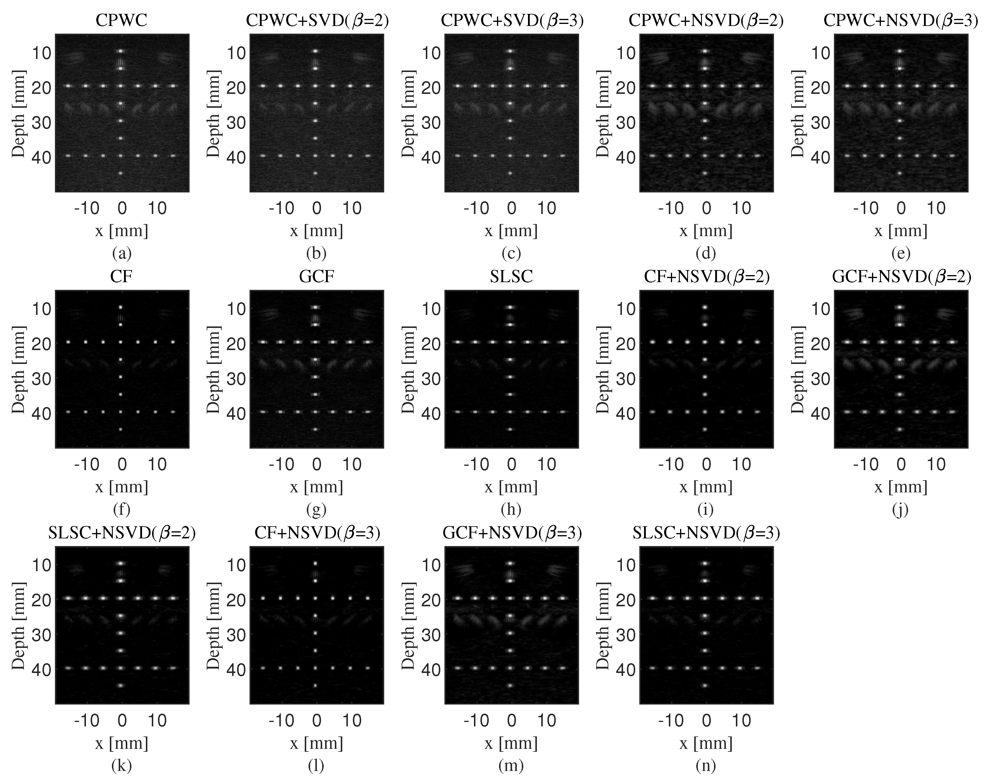
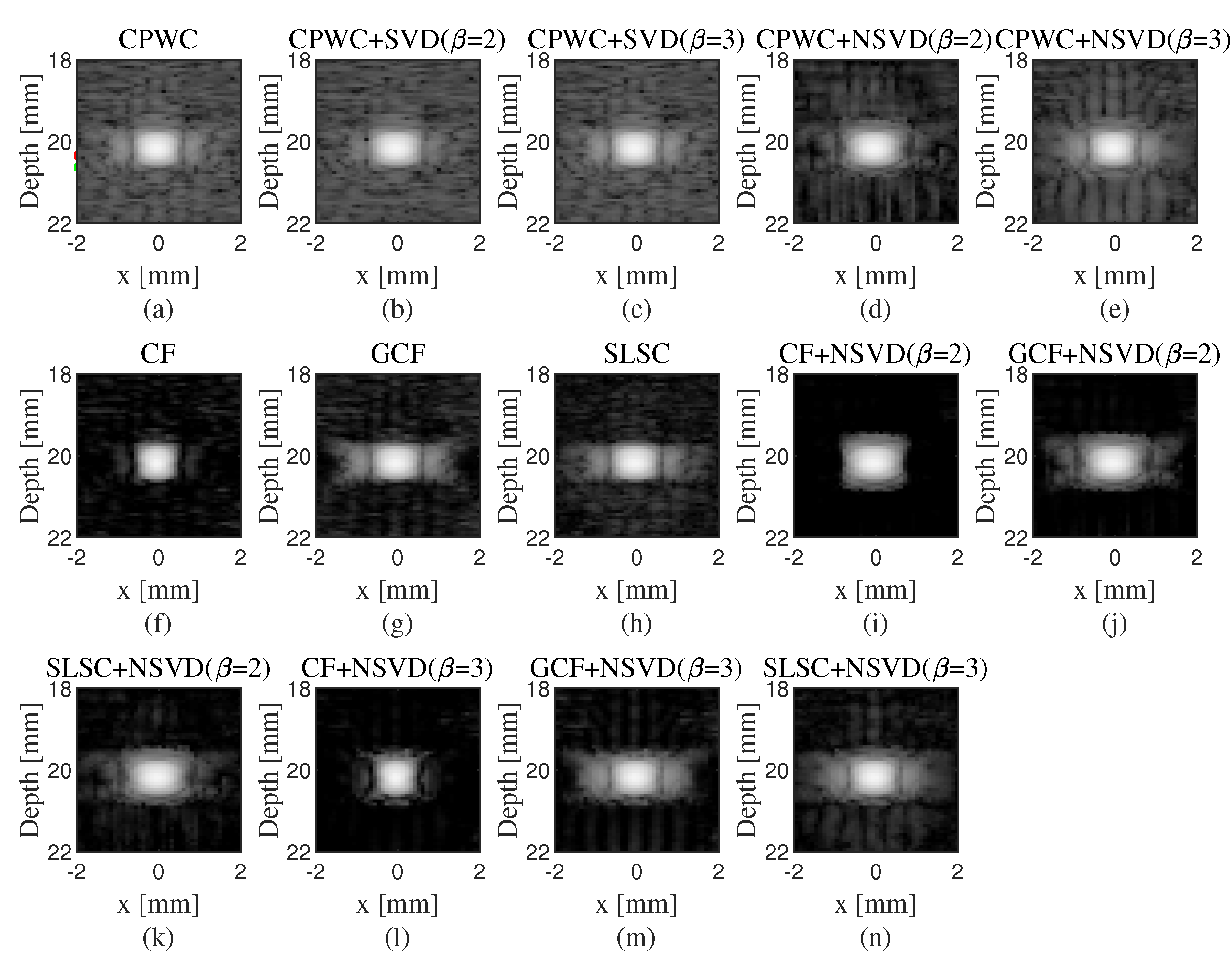
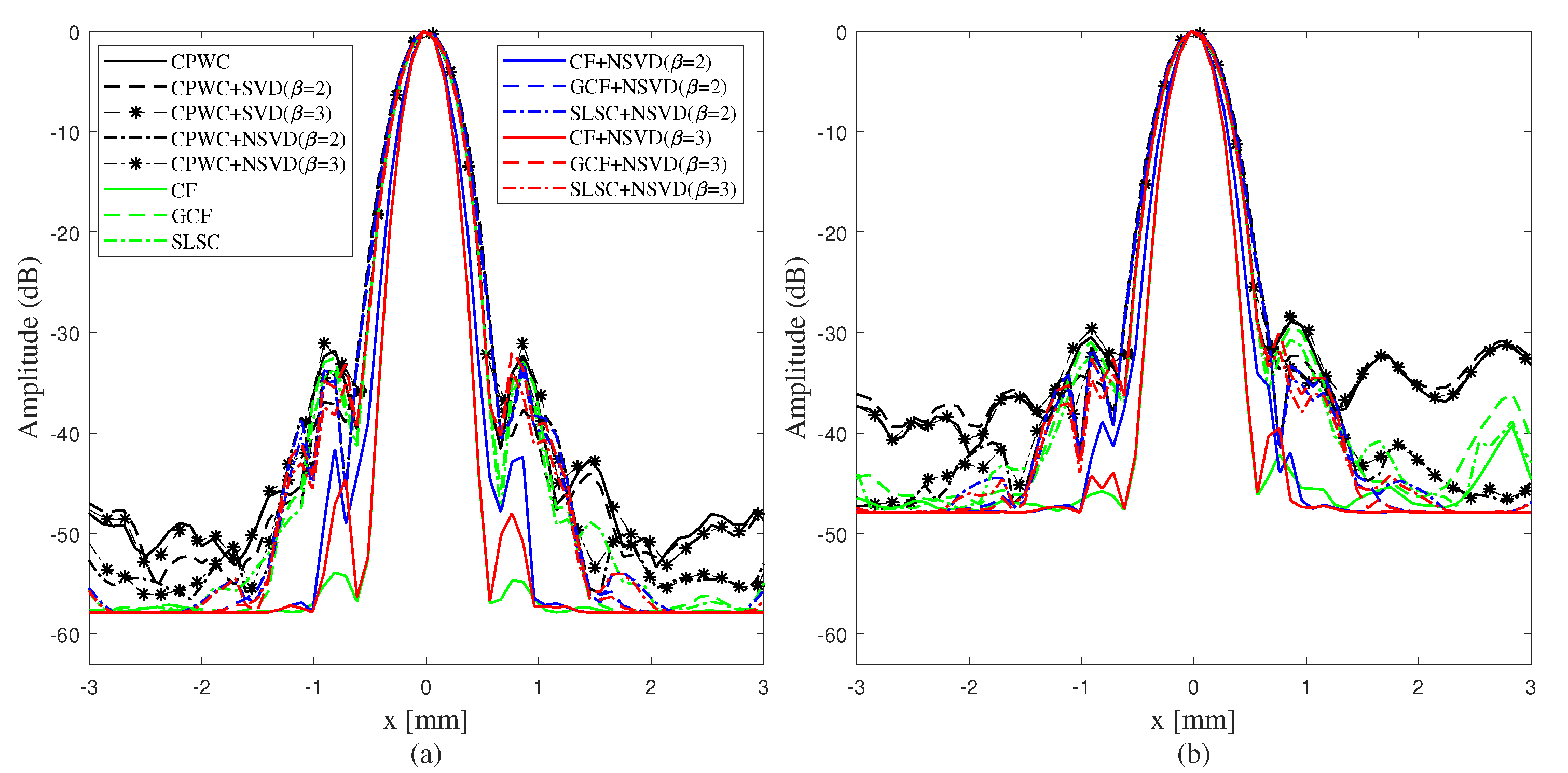
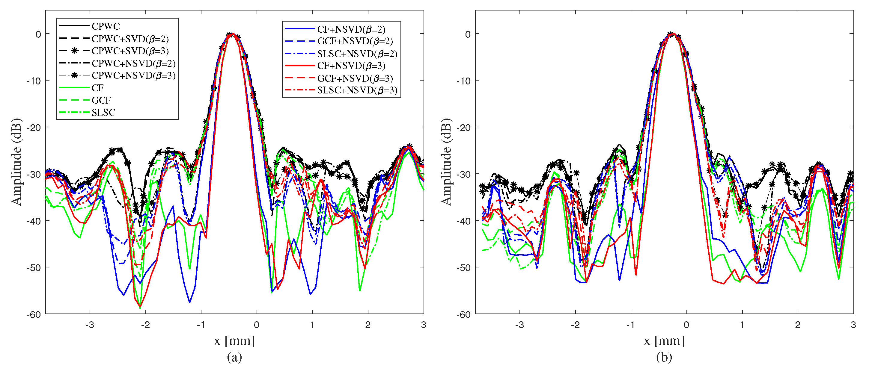
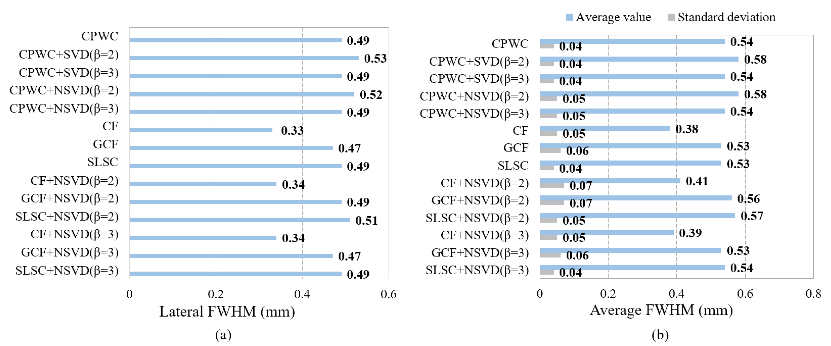
4.1.1. Simulated Phantom with Point Targets

The proposed CPWC+NSVD method was compared to CPWC and CPWC+SVD. Images obtained using adaptive weighting factors (CF, GCF, and SLSC) to weight the output of CPWC were also presented as a comparison of the adaptive weighting methods based on NSVD. For convenience, hereinafter, CPWC weighted by CF, GCF, and SLSC are referred to as CF, GCF, and SLSC, respectively.
The first simulated phantom contains several point targets from a depth of 10 mm to 45 mm. Figure 1 presents B-mode images beamformed using different methods. The top row contains CPWC, CPWC+SVD, and CPWC+NSVD images. The second and third rows contain CF-, GCF-, and SLSC-weighted CPWC images and weighted images with the NSVD filter for β = 2 and β = 3 . Figure 2 shows the zoomed images of the point target located at a depth of 20 mm with a dynamic range of 80 dB. CPWC shows the highest noise and sidelobe levels. Through the use of the NSVD filter, noise is suppressed in the images of Figure 1d–e and Figure 2d–e, while sidelobes of NSVD+CPWC show little suppression compared to CPWC. It is also noted that the adaptive weighting methods can reduce noise and sidelobes relative to CPWC, CPWC+SVD, and CPWC+NSVD. Lateral profiles of two-point targets p 1 ( x , z ) = ( 0 mm, 20 mm) and p 2 ( x , z ) = ( 0 mm, 40 mm) in all simulated images are shown in Figure 3. For adaptive weighting methods, the NSVD filter leads to increased sidelobes, which is obvious in CF-weighted images. After further observations, NSVD+CPWC shows reduced sidelobes compared to CPWC and CPWC+SVD in Figure 2b. Therefore, NSVD may have a good ability to suppress sidelobes in the deep region. It is also observed that beamformers with β = 3 provide narrower mainlobes than those with β = 2 .
The lateral FWHM of point targets p 1 ( x , z ) = ( 0 mm, 20 mm) and the average FWHM of all simulated point targets are calculated and Figure 4 gives the barplot of lateral FWHM. As seen in Figure 4, the NSVD filter has little effect on lateral FWHM. Compared to CPWC, CPWC+SVD ( β = 2 ) and CPWC+NSVD ( β = 2 ) have a slightly larger lateral FWHM, while CPWC+SVD ( β = 3 ) and CPWC+NSVD ( β = 3 ) have equivalent lateral FWHM values. For adaptive weighting methods, β = 2 also leads to a wider lateral FWHM.

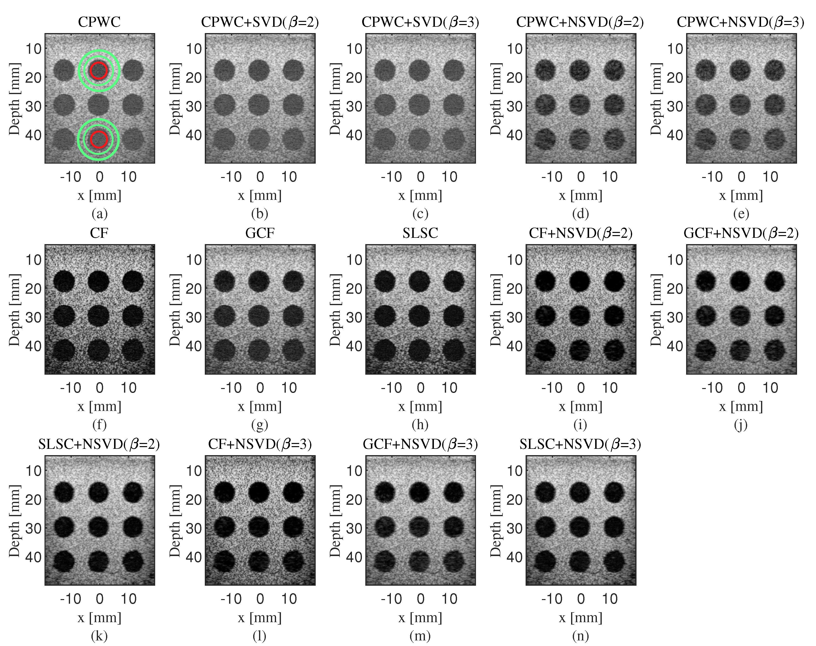
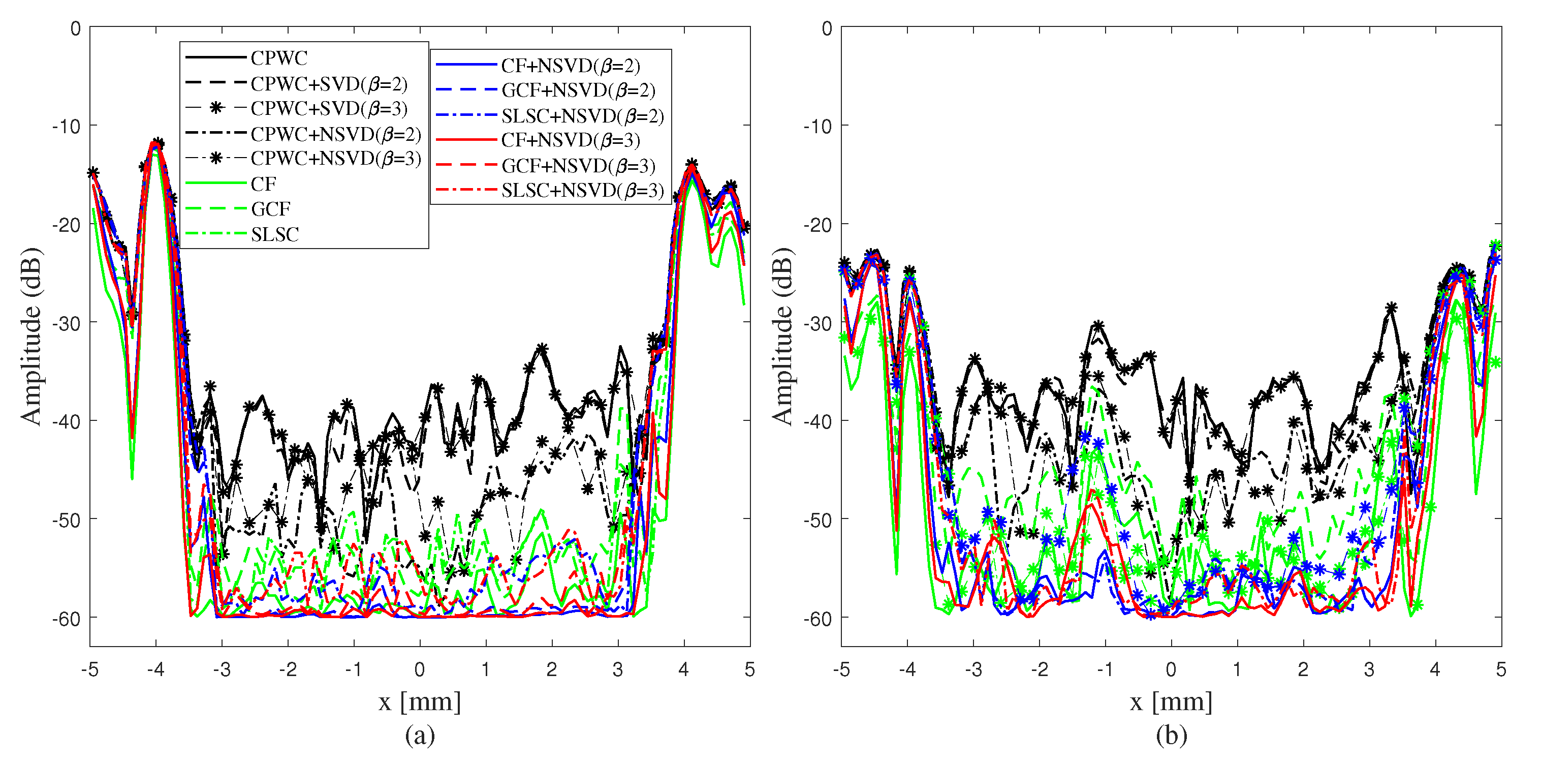
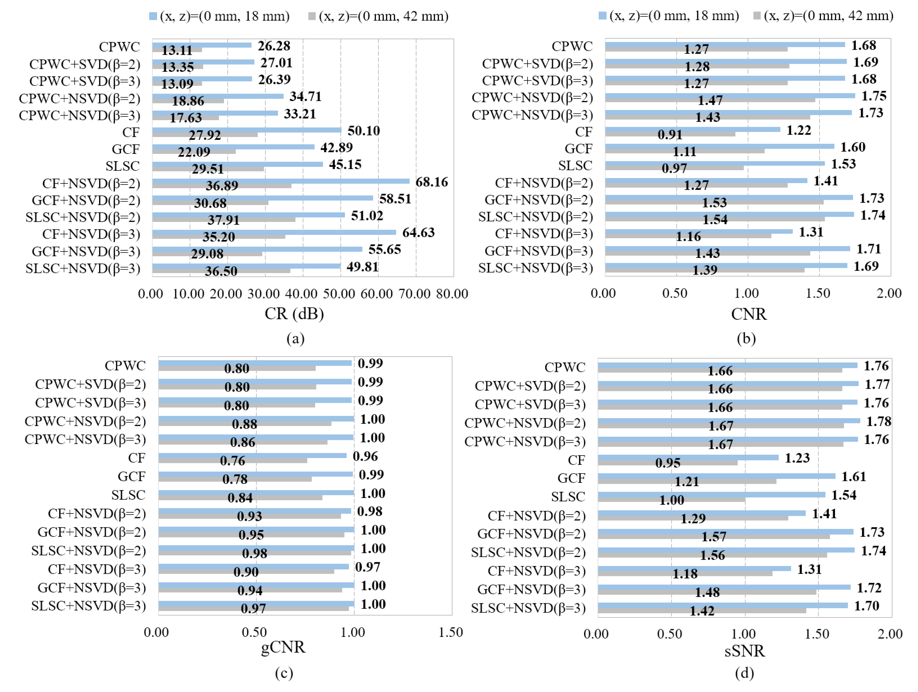
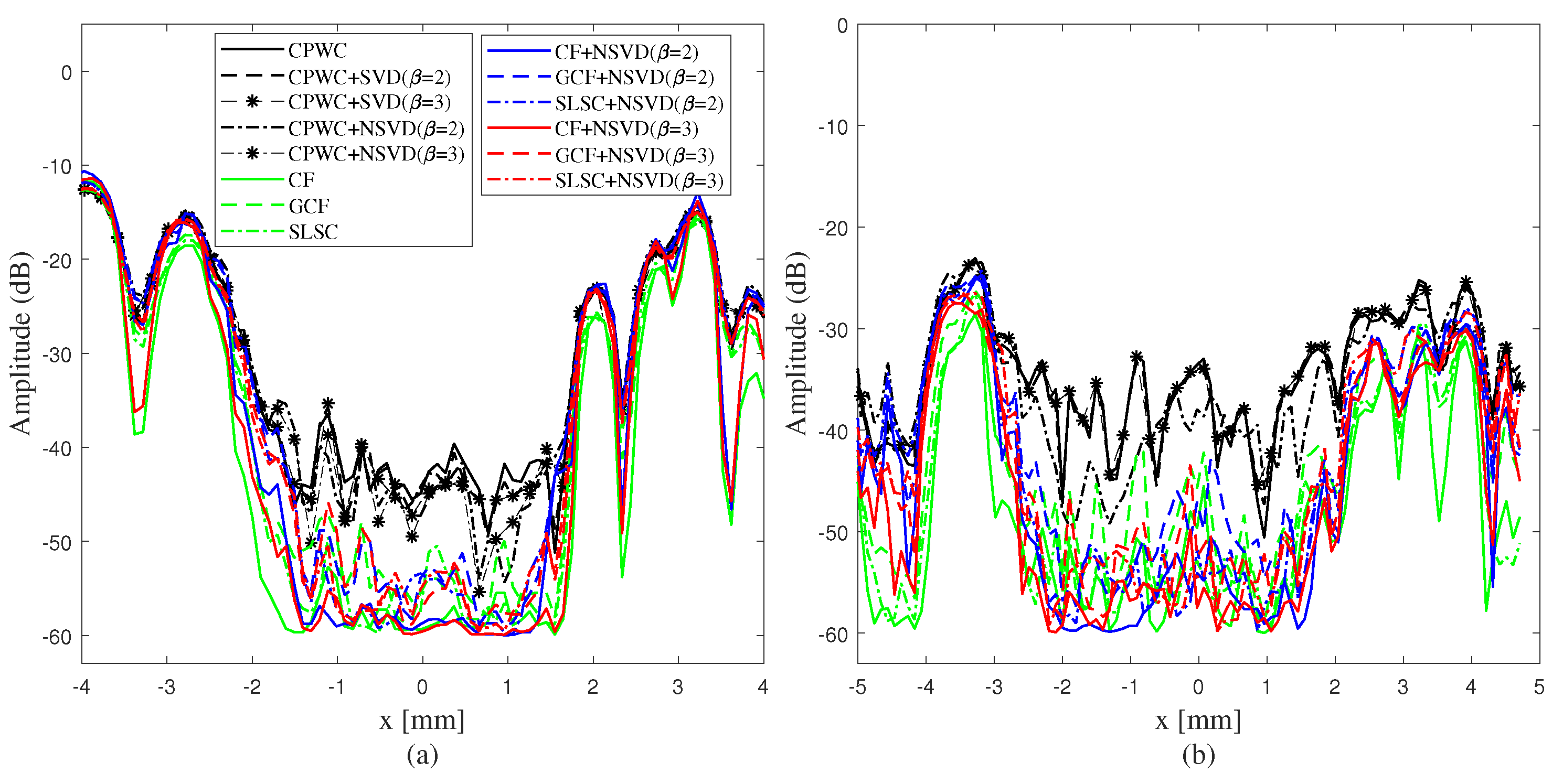
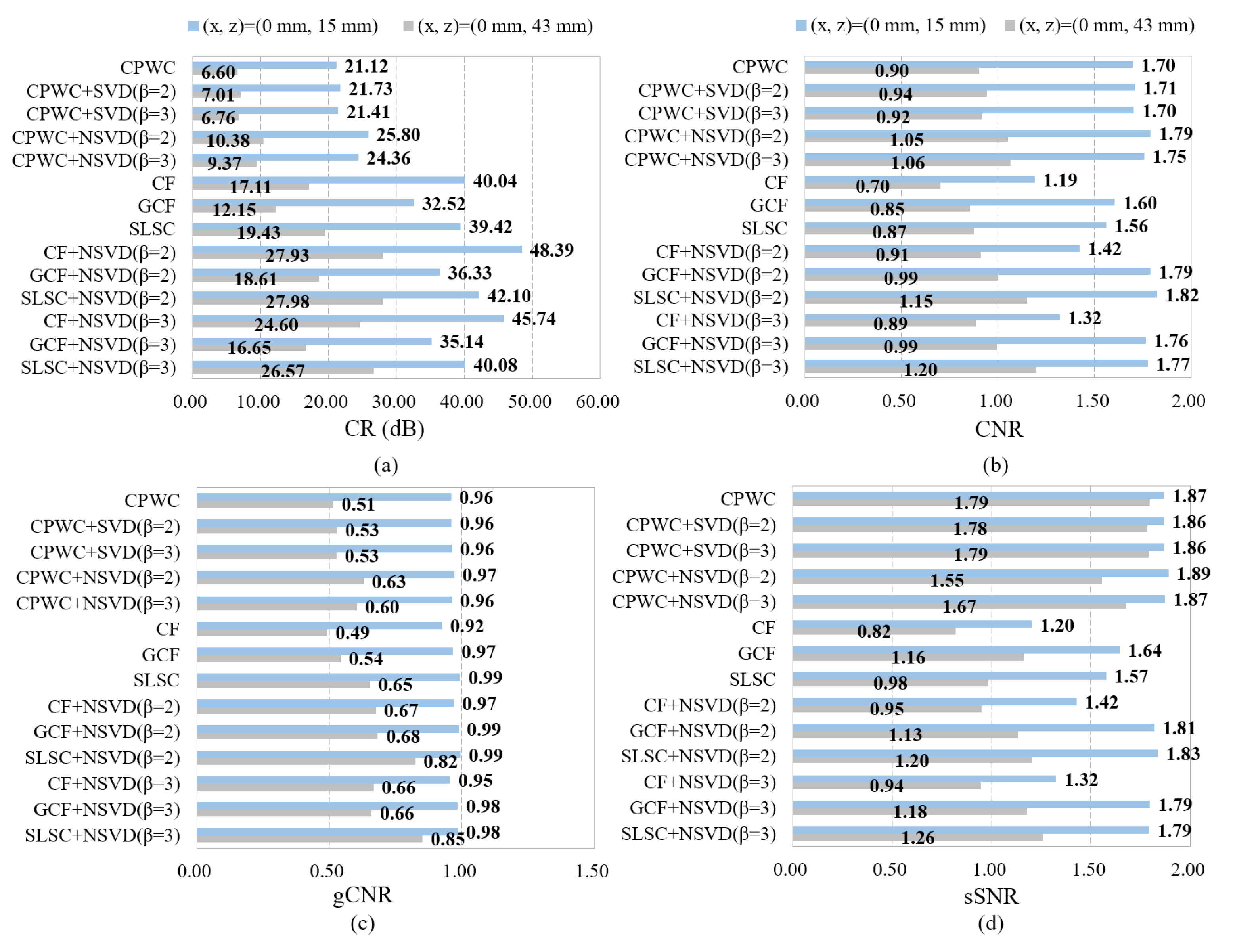
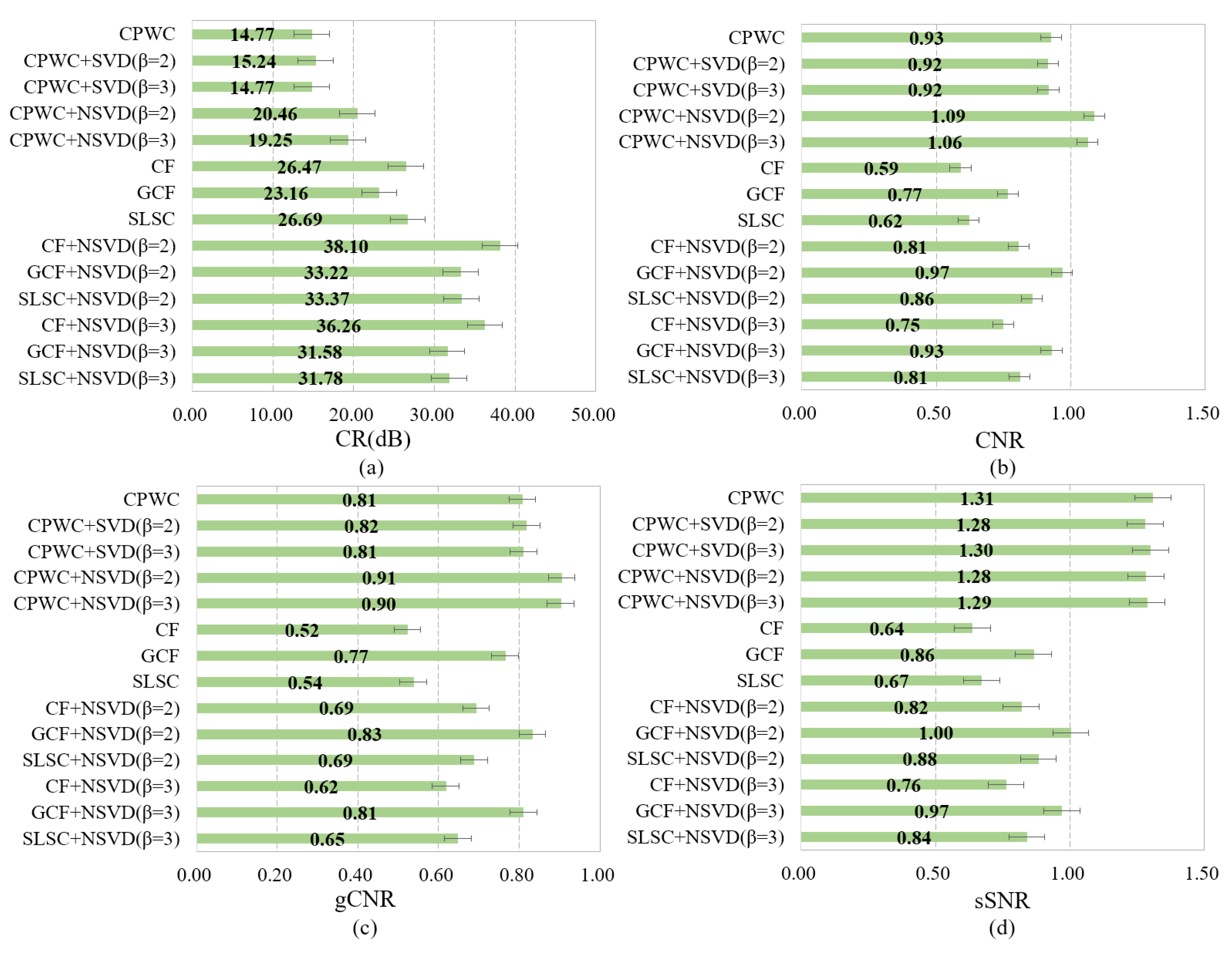
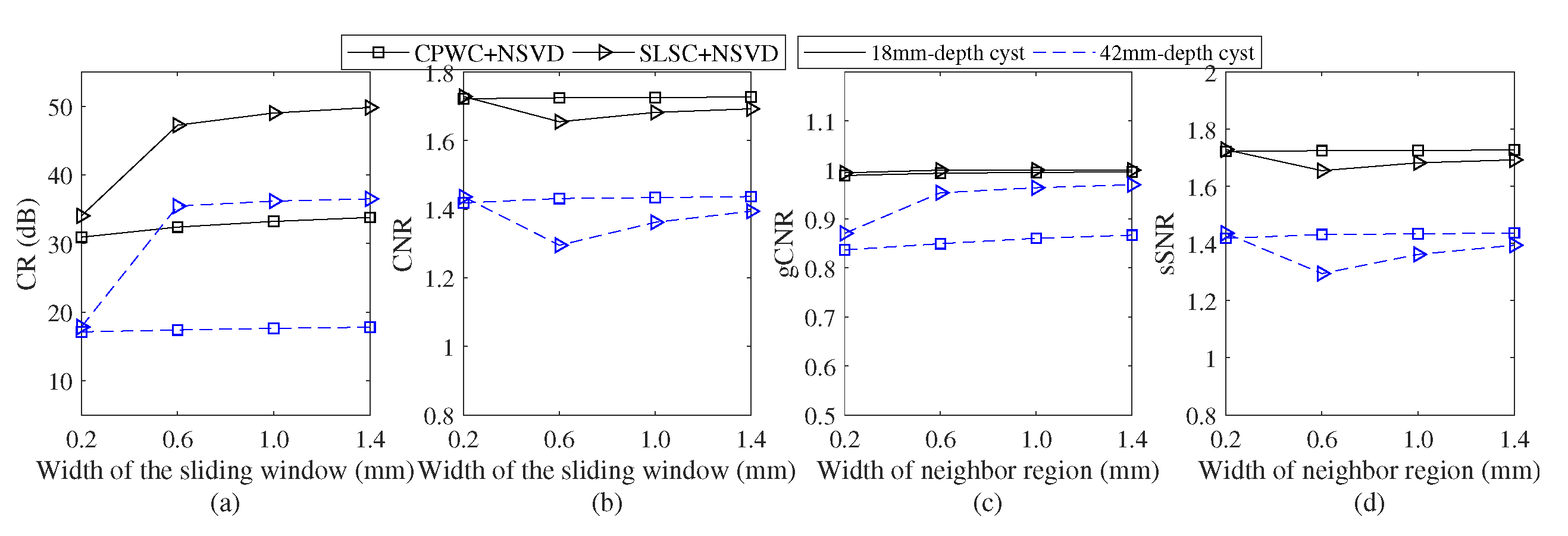
4.1.2. Simulated Cyst Targets

The second simulated phantom contains anechoic cysts and a homogeneous speckle background. Figure 5 presents the simulated cyst target images reconstructed by various methods. Anechoic cysts in the CPWC+NSVD images of Figure 5d–e have less noise than the CPWC and CPWC+SVD images of Figure 5a–c. Compared to Figure 5f–h, the corresponding Figure 5i–k and Figure 5l–n show reduced dark-region artifacts in the background speckle and higher background intensity. Figure 6 displays the lateral profiles of two cyst targets centered at depths of 18 mm and 42 mm and distributed at the middle line ( x = 0 mm) in Figure 5. The CPWC+NSVD shows reduced noise inside the anechoic cysts as compared to CPWC and CPWC+SVD. Similarly, when combined with the NSVD filter, the adaptive weighting methods also show better noise suppression.
In Figure 5a, we indicate the marked regions used to calculate CR, CNR, gCNR, and sSNR, according to Equations (19)–(22). Being within the red circle means inside the cyst, while being within the two green circles means inside the background speckle. Figure 7 gives the barplot of the quantified values for each method. CPWC+NSVD has improved CR and CNR values relative to CPWC. Compared to CPWC, CPWC+NSVD ( β = 3 ) can achieve CR improvements of 6.93 dB/4.52 dB (26.4%/34.5%) and CNR improvements of 0.05/0.16 (3%/12.3%). The adaptive weighting methods based on NSVD all have improved CR, CNR, and sSNR. CF+NSVD ( β = 3 ) has improvements of 14.53 dB/7.28 dB (29%/26.1%) in CR, 0.09/0.25 (7.4%/27.5%) in CNR, and 0.08/0.23 (6.5%/24.2%) in sSNR. The CR, CNR, and sSNR improvements of GCF+NSVD ( β = 3 ) are 12.76 dB/6.99 dB (29.8%/31.6%), 0.11/0.32 (6.9%/28.8%), and 0.11/0.27 (6.8%/22.3%). The corresponding improvements of SLSC-NSVD ( β = 3 ) are 4.66 dB/6.99 dB (10.3%/23.7%), 0.16/0.42 (10.5%/43.3%), and 0.16/0.42 (10.4%/42%), respectively. In the near region, gCNR values of different methods are similar. For the deep region, the NSVD leads to a gCNR improvement by about 0.14 for adaptive weighting methods. It can be observed that β has an effect on CR, CNR, gCNR and sSNR. For adaptive weighting methods, NSVD ( β = 2 ) leads to improvements of CR, CNR, and sSNR by about 2 dB, 0.1, and 0.1 compared with NSVD ( β = 3 ), respectively.

4.2. Phantom Experiment

4.2.1. Experimental Phantom with Point Targets

The first experimental phantom contains point targets, a massive cyst, and a speckle background. Figure 8 presents images of the experimental phantom with point targets beamformed by various beamformers. Images obtained by adaptive weighting methods show dark artifacts beside point targets compared to CPWC, CPWC+SVD, and CPWC+NSVD. GCF and SLSC provide fewer artifacts than CF. From Figure 8i–k, these dark artifacts become more visible through the use of the NSVD ( β = 2 ) filter. However, in adaptive weighting images, NSVD ( β = 3 ) results in reduced artifacts compared to NSVD ( β = 2 ). Images of GCF+NSVD ( β = 3 ) and SLSC+NSVD ( β = 3 ) show fewer dark artifacts than other adaptive weighting methods.
Figure 9 plots the lateral profiles of two experimental point targets positioned at p 1 ( x , z ) = ( 0 . 4 mm, 18 mm) and p 2 ( x , z ) = ( 0 . 4 mm, 38 mm). As seen in Figure 9, CPWC+SVD and CPWC+NSVD have slightly lower sidelobes than CPWC. Experimental point targets of adaptive weighting methods show narrowed mainlobes and suppressed sidelobes compared to CPWC, CPWC+SVD, and CPWC+NSVD. Figure 10 shows the barplot of the quantitative lateral FWHM of the experimental point targets. Adaptive weighting methods can significantly improve the lateral resolution. The NSVD filter has only a slight effect on lateral FWHM and increased β results in decreased lateral FWHM, which is consistent with the simulation results.

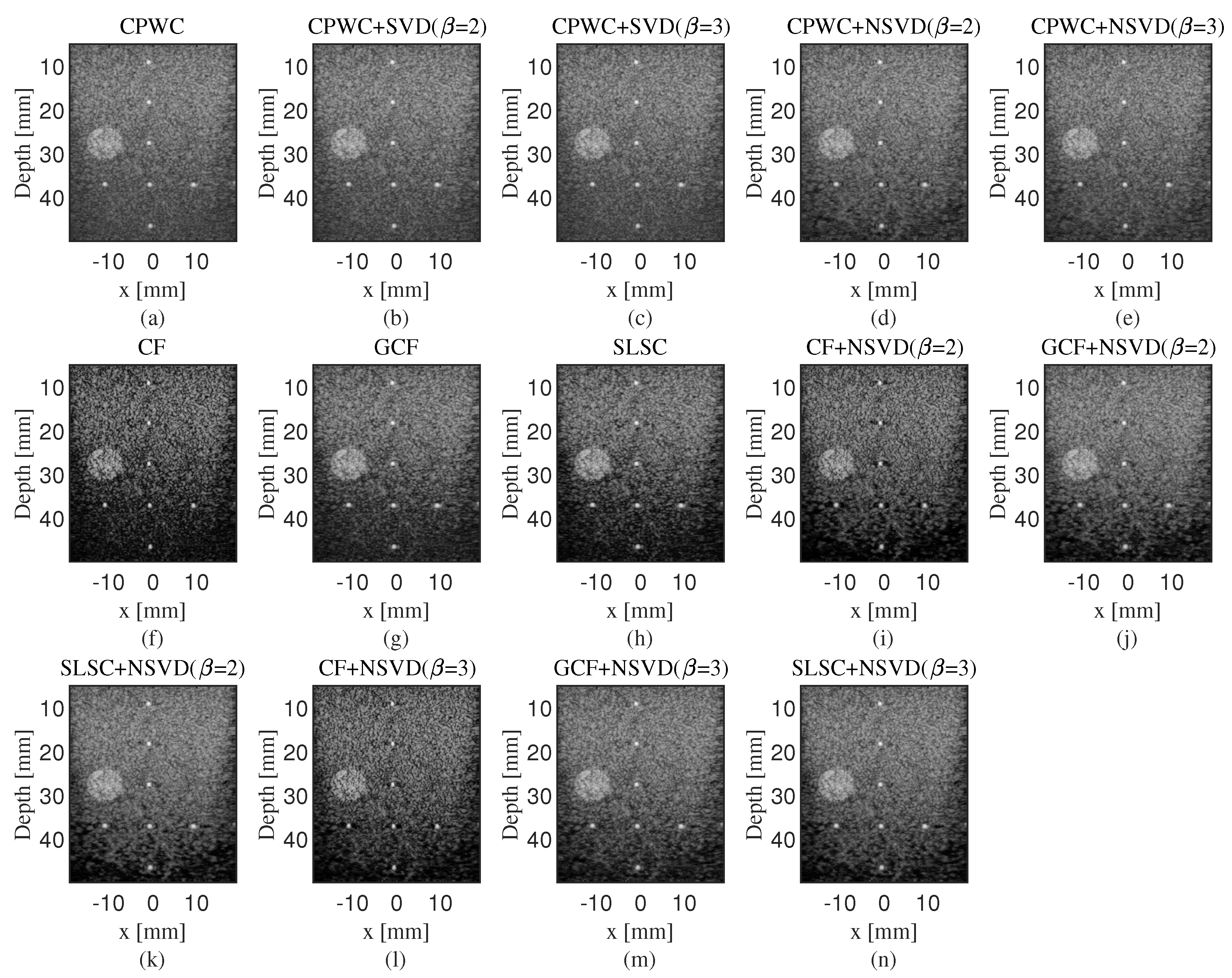
4.2.2. Experimental Cyst Targets

The second experimental phantom contains two anechoic cyst targets and a speckle background. The B-mode images of the experimental phantom with cyst targets obtained by different beamformers are shown in Figure 11. It can be observed that anechoic cysts in the CPWC+NSVD image have less noise than with CPWC+SVD. Adaptive weighting methods achieve improved image quality because, in their images, noise is suppressed and the boundaries of cyst targets are more easily detectable. However, the images of adaptive weighting methods show visible dark-region artifacts in the background speckle and the image intensity is reduced, especially in the deep region. With the combination with NSVD, in the near region, all the adaptive weighting methods provide reduced dark-region artifacts in the speckle and obtain brighter background speckle. For the deep region, dark-region artifacts become worse in images of adaptive weighting methods with NSVD ( β = 2 ). However, when β = 3 , the artifacts in the deep region are reduced and the speckle pattern in the near region is still well-preserved.
Figure 12 presents the lateral profiles of the two experimental cysts. It is also observed that CPWC+NSVD has an advantage in terms of noise suppression over CPWC and CPWC+SVD. Figure 13 presents the barplot of CR, CNR, and sSNR in experimental cyst target images. CPWC+NSVD outperforms CPWC+SVD and CPWC in terms of CR, and CNR. Compared to CPWC, CPWC+NSVD ( β = 3 ) achieves CR improvements of 3.24 dB/2.77 dB (15.3%/42%), and CNR improvements of 0.05/0.16 (3%/17.8%). For CF, by combining with the NSVD filter, CR, CNR, and sSNR achieve improvements of 5.7dB/7.49 dB (14.2%/43.8%), 0.13/0.19 (10.9%/27.1%), and 0.12/0.12 (10%/14.6%), respectively. For the GCF ( β = 3 ), the corresponding improvements are 2.62 dB/4.5 dB (8.1%/37%), 0.16/0.14 (10%/16.5%), and 0.15/0.02 (9.2%/1.7%), while for the SLSC ( β = 3 ), the corresponding improvements are 0.66 dB/7.14 dB (1.7%/36.8%), 0.34/0.33 (23.8%/37.9%), and 0.35/0.28 (24.3%/28.6%), respectively. The gCNR improvements in the deep region are more than 0.1 due to the utilization of NSVD. For adaptive weighting methods, NSVD ( β = 2 ) and NSVD ( β = 3 ) both achieve enhancements of CR, CNR, gCNR, and sSNR. This indicates that adaptive methods can achieve improved image contrast and quality of speckle pattern by combining with the NSVD filter.

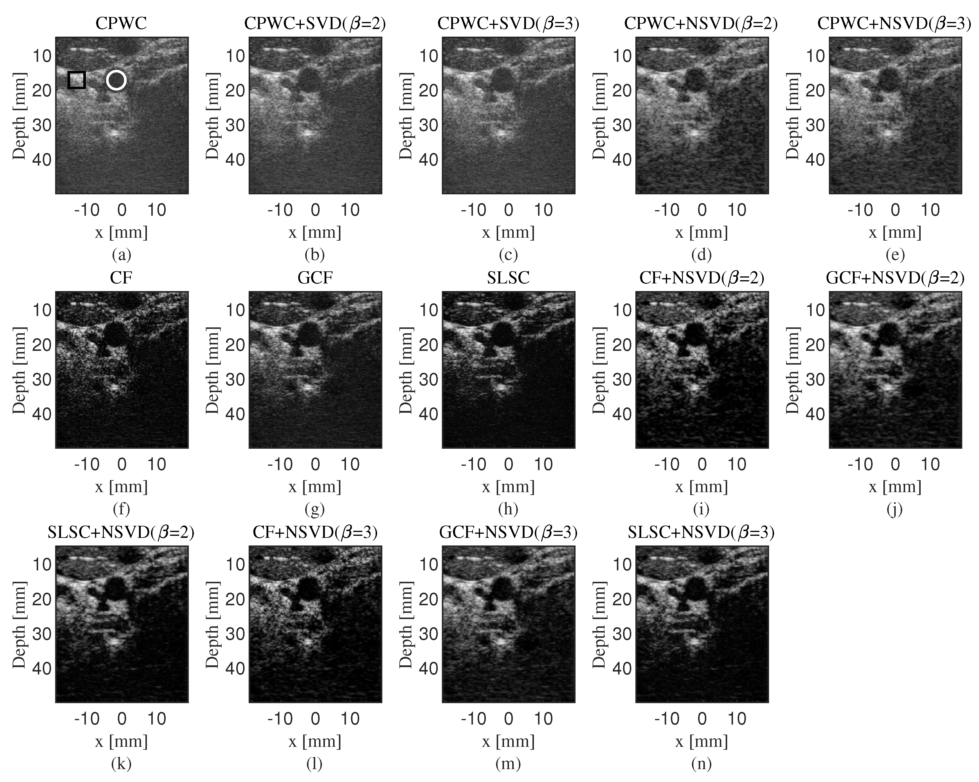
4.3. In Vivo Experiment

All presented methods were next applied to in vivo datasets obtained from a human carotid artery. In vivo images obtained with various beamformers are shown in Figure 14. The adaptive weighting methods of Figure 14f–n show clear carotid arteries with little noise. As observed, CPWC+NSVD outperforms CPWC and CPWC+SVD in terms of reduced noise inside the carotid. Adaptive weighting methods provide visible noise suppression inside the carotid. However, the speckle pattern is affected relative to CPWC. Due to the combination of the NSVD filter, enhanced noise suppression and speckle preservation can be achieved for all the adaptive methods.
Various parameters are used to verify the efficiency of different methods. A circular region inside the carotid artery and a rectangular region outside the carotid artery are marked in Figure 14a and used to calculate CR, CNR, and sSNR. Figure 15 show the barplot of quantitative results. CPWC+NSVD achieves a CR enhancement (over 5 dB) and similar CNR and sSNR compared to CPWC. The adaptive weighting methods combined with the NSVD filter can obtain CR improvements (by about 8 dB), as well as improved CNR, gCNR, and sSNR.

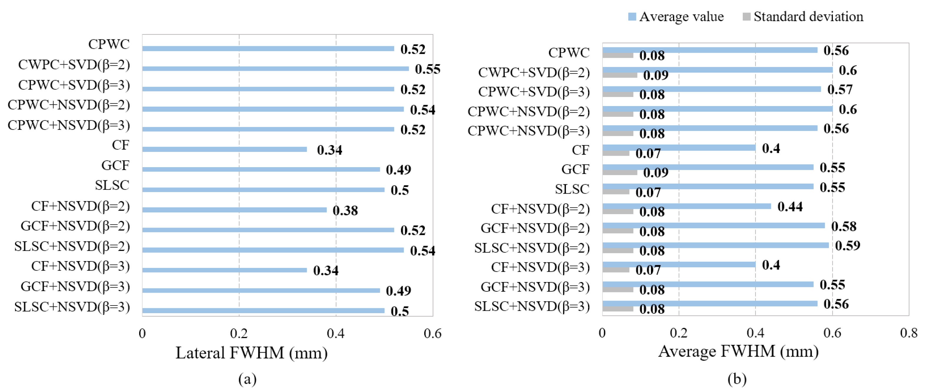
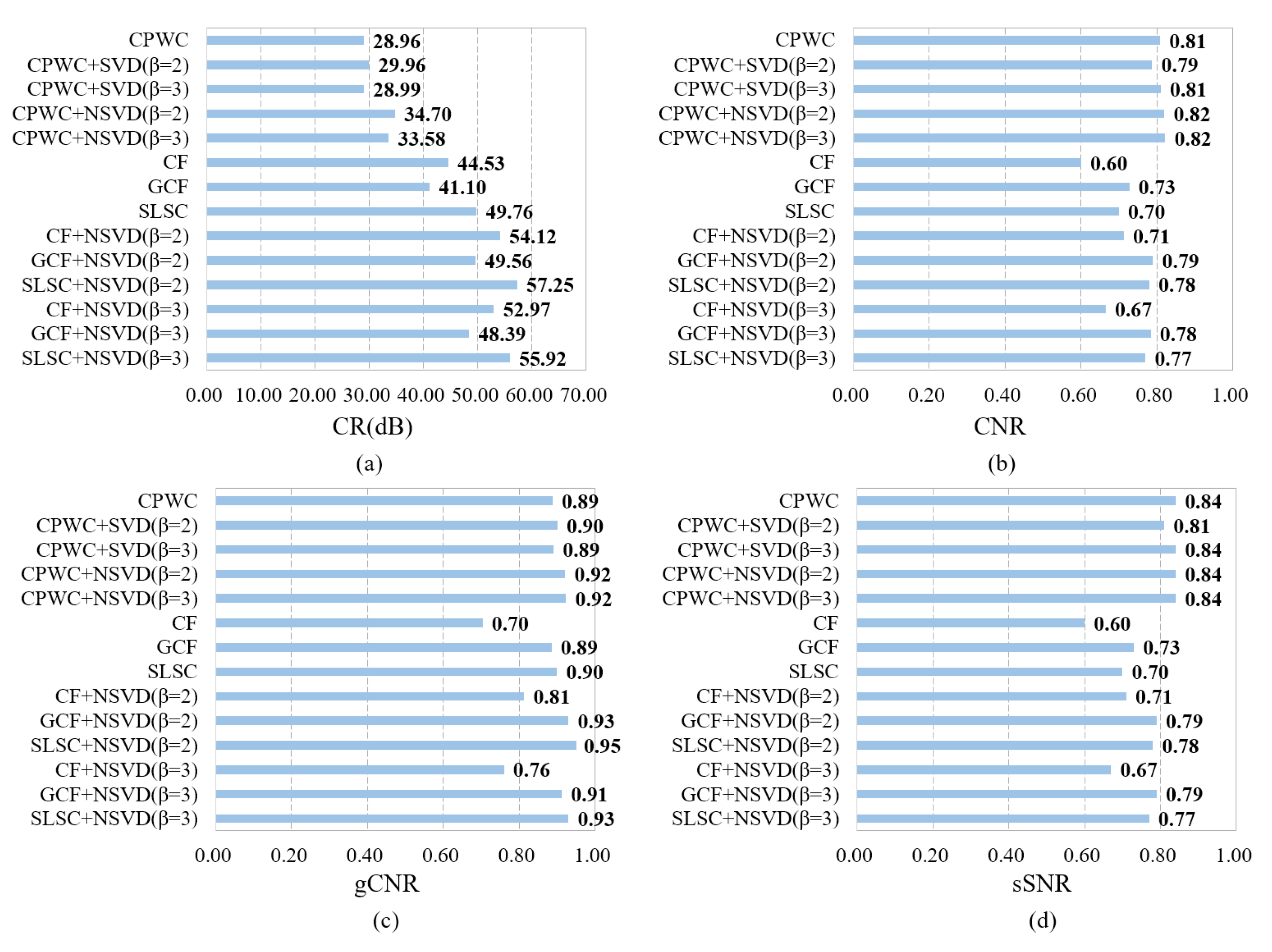
4.4. Statistical Analysis of Results

We use the t-test to determine whether there is a significant statistical difference between quantitative metrics calculated for different methods. Lateral FWHM, CR, CNR, gCNR, and sSNR calculated in all simulated and experimental images are used to evaluate the significant improvements of proposed methods. A paired t-test was performed between NSVD-based methods and methods without the use of NSVD at a 5% significance level. The results indicate that NSVD does not effectively help the lateral FWHM. However, compared to CPWC and CWPC+SVD, the CR and CNR improvements obtained by CPWC+NSVD are significant. Furthermore, CF+NSVD, GCF+NSVD, and SLSC+NSVD show significant improvements of CR, CNR, gCNR, and sSNR compared with corresponding CF, GCF, and SLSC, respectively.
Because of the complicated tissue in in vivo images, the overall improvement of NSVD is hard to judge using only the results in Figure 15. We chose several different background regions to calculate metrics and statistically assess significant improvement. Figure 16 shows the barplot of CR, CNR, and sSNR of in vivo images obtained by different imaging methods. The results of the paired t-test at a 5% significance level show the significant improvements in CR and CNR of CPWC+NSVD as compared to CPWC and CPWC+SVD, while CR, CNR, gCNR, and sSNR improvements are also significant between an adaptive weighting method with NSVD and without the use of NSVD.

5. Discussion

Here, we proposed a neighborhood singular value decomposition (NSVD) filter and its combination with adaptive weighting methods for CPWC to improve imaging performance (noise reduction and speckle pattern preservation). The center-surround relation is useful since the surrounding region has more correlations and gives more useful clues for an imaging point. NSVD considers information of the neighbor region instead of the entire region so that it can more accurately reserve effective signals and reduce noises. The main characteristic of the NSVD filter is that it uses a sliding rectangular window to slice the entire region into several continuous sub-regions, then performs SVD for all sub-regions. The sliding window can be viewed as a smoothing filter with a step of 1. Therefore, the NSVD filter actually has the advantages of the SVD filter and smoothing filter. To verify the performance of the NSVD filter, lateral FWHM, CR, CNR, gCNR, and sSNR are assessed in simulation and experiments. Our results indicate that the NSVD filter has little effect on the lateral resolution. However, it does help to reduce noise and can improve the quality of speckle pattern of images beamformed using adaptive weighting methods. Compared to CPWC and CPWC+SVD, CPWC+NSVD can obtain higher CR and CNR. By combining with the NSVD filter, CF, GCF, and SLSC all provide improved CR, CNR, gCNR, and sSNR.
The SVD filter can reduce sidelobes and maintain mainlobes due to the high coherence of mainlobe signals and the high incoherence of sidelobe signals, while the number of eigenvalues, β , will affect the performance of the SVD filter. As per Figure 4b–c, a smaller β leads to lower sidelobes but a wider mainlobe, which is the same as with the NSVD filter. Therefore, the NSVD filter can hardly reduce the mainlobe width, and thus produces no improvement in the lateral resolution. From both simulated and experimental data, NSVD-based methods achieve a better image contrast than those methods without the use of NSVD, since noises within cysts are further suppressed, as shown in Figure 6, Figure 12 and Figure 15. It can be seen from the B-mode images that adaptive weighting methods influence the speckle pattern. Images of CF, GCF, and SLSC show visible dark-region artifacts and low CNR and sSNR compared to the CPWC image. Multiple studies have indicated that adaptive beamforming methods alter the statistical distribution of the speckle and increase the variance of the background speckle pattern [27,42], which can be reflected from the degraded sSNR. However, using the NSVD filter in adaptive weighting methods, we can observe decreased dark-region artifacts and background variance in B-mode images, since the NSVD filter has the characteristic of smoothing images. It is also demonstrated that CF+NSVD, GCF+NSVD, and SLSC+NSVD provide higher CNR and sSNR than the corresponding CF, GCF, and SLSC (Figure 7, Figure 13 and Figure 15). From all B-mode images, we see that SLSC+NSVD ( β = 3 ) suffers from few artifacts and provides outstanding performance in terms of CR, CNR, gCNR, and sSNR. Therefore, among the methods of CF+NSVD, GCF+NSVD, and SLSC+NSVD, we recommend SLSC+NSVD with β = 3 as the best overall method.
The width of the sliding window (i.e., the size of the neighbor region) and β both have an influence on the imaging performances of the proposed methods. From Figure 17, NSVD-based methods achieve stable CR, CNR, gCNR, and sSNR when the width of the sliding window is larger than 1.6 mm. It should be noted that a wide window for NSVD will increase the computational load. As mentioned, NSVD tends to utilize the neighbor region clues, thus it may not be reasonable to select a large sliding window. From the simulation and experimental results, NSVD with both β = 2 and β = 3 can improve the image quality in CR, CNR, gCNR, and sSNR. However, experimental images obtained by adaptive weighting methods with NSVD ( β = 2 ) show severe dark artifacts alongside point targets and in the deep region. Figure 18 and Figure 19 presents the effect of the β value on the image quality. It can be seen that all values of these metrics increase as β decreases. Nevertheless, artifacts alongside point targets become more visible with a small β . Generally, these artifacts can be reduced by increasing β . Therefore, β = 3 is a suitable choice for the application of NSVD.
To evaluate the impact of the number of plane-waves on the quality of compounded images obtained by the proposed methods, we performed several tests using simulated cyst data and calculated the CR, CNR, and sSNR. SLSC ( β = 3 ) is used as a representation of adaptive weighting methods, and β = 3 is used for SVD and NSVD. Figure 20 shows a comparison of different methods. CR and CNR increase as the number of compounding angles increases, while sSNR is relatively stable. When decreasing the number of compounded plane-waves, CPWC+NSVD can still provide higher CR and CNR than CPWC and CPWC+SVD. It is also observed that the CPWC+NSVD with 25 plane-waves can achieve comparable performance to CPWC with 75 plane-waves in CR, CNR, and sSNR. The SLSC ( β = 3 ) has a consistent variation, as shown in Figure 18. For both the near and deep regions, SLSC+NSVD outperforms SLSC in CR, CNR, and sSNR.
Since the simulated and experimental phantoms usually have omnidirectional scatters and uniform propagation velocity, the influence of angle dependency on simulated and experimental images would not be apparent. For human tissue imaging, the echo signals include coherent backscattered signals from the focal plane and incoherent reverberation clutter signals [43]. Coherent signals show high coherence between different transmit angles, while reverberation clutter signals show high angle-dependency. This indicates that the influence of transmitting angles may be more apparent in the in vivo image compared to simulated and experimental images. Therefore, we also present the effect of plane-wave numbers on the image quality metrics of in vivo images in Figure 21. Similar to the simulation case, 25 plane-waves are required for CPWC+NSVD to provide equivalent CR, CNR, and sSNR compared to CPWC, with 75 plane-waves. With an equal number of plane-waves, SLSC+NSVD shows improved image quality compared to SLSC in terms of CR, CNR, and sSNR.
The SVD filter was performed for the entire image, while the NSVD is a pixel-based filter. For each imaging point in an image, NSVD must perform an SVD filter for a neighbor region centered at the imaging point. Therefore, the computational complexity of NSVD is higher compared to SVD. We recorded the runtime of SVD ( β = 3 ) and NSVD ( β = 3 ) using simulated datasets on a PC with an Intel(R) Core(TM) i7-7700HQ CPU at 2.8 GHz and RAM of 8 GB. The number of plane-waves was 25, and each image contained 3328 × 387 pixels. SVD and NSVD required a runtime of 0.32 s and 149.62 s, respectively.

6. Conclusions

We propose an NSVD filter and study its application in adaptive beamforming for high-quality CPWC images. The proposed CPWC+NSVD method is compared to CPWC and CPWC+SVD on simulated and experimental datasets, while CF, GCF, and SLSC are presented to show the image quality improvements when the NSVD filter is combined with adaptive weighting factors. We found that CPWC+NSVD outperforms CPWC and CPWC+SVD in noise suppression, which provides higher CR and CNR. With 25 plane-waves, CPWC+NSVD achieves similar CR, CNR, and sSNR compared to CPWC with 75 plane-waves. When applied in combination with adaptive beamforming methods, the NSVD filter helps to achieve a well-preserved speckle pattern and further reduce noise. We also analyze the influences of the size of the sliding window (i.e., neighbor region) and β values on the proposed methods. We recommend the size of neighbor region about 1 mm and β = 3 by taking into consideration of image quality and computational complexity. Regarding the optimization of computational efficiency, parallel computation can be adopted to improve imaging speed.

Author Contributions

Conceptualization, S.F.; methodology, S.F. and Y.W.; software, S.F.; validation, Y.W.; formal analysis, S.F., Y.W., and C.Z.; investigation, S.F. and Y.W.; writing—original draft preparation, S.F. and Y.W.; writing—review and editing, S.F., Y.W., C.Z., Z.H., and H.P.; visualization, S.F.; supervision, C.Z., Z.H., and H.P.; project administration, C.Z., Z.H., and H.P.; funding acquisition, Z.H. and H.P. All authors have read and agreed to the published version of the manuscript.

Funding

This research was funded by the National Natural Science Foundation of China, grant numbers 61501163 and 61172037.

Acknowledgments

The authors are grateful to the Plane-wave Imaging Challenge in Medical Ultrasound (PICMUS) organizers for sharing imaging data.

Conflicts of Interest

The authors declare no conflict of interest.

References

  1. Kang, J.; Jang, W.S.; Yoo, Y. High PRF ultrafast sliding compound doppler imaging: Fully qualitative and quantitative analysis of blood flow. Phys. Med. Biol. 2018, 63, 045004. [Google Scholar] [CrossRef]
  2. Couture, O.; Fink, M.; Tanter, M. Ultrasound contrast plane wave imaging. IEEE Trans. Ultrason. Ferroelectr. Freq. Control. 2012, 59, 2676–2683. [Google Scholar] [CrossRef]
  3. Errico, C.; Pierre, J.; Pezet, S.; Desailly, Y.; Lenkei, Z.; Couture, O.; Tanter, M. Ultrafast ultrasound localization microscopy for deep super-resolution vascular imaging. Nature 2015, 527, 499–502. [Google Scholar] [CrossRef]
  4. Lu, J.Y. 2D and 3D high frame rate imaging with limited diffraction beams. IEEE Trans. Ultrason. Ferroelectr. Freq. Control 1997, 44, 839–856. [Google Scholar] [CrossRef]
  5. Lu, J.Y. Experimental study of high frame rate imaging with limited diffraction beams. IEEE Trans. Ultrason. Ferroelectr. Freq. Control 1998, 45, 84–97. [Google Scholar] [CrossRef] [Green Version]
  6. Schiffner, M.F.; Jansen, T.; Schmitz, G. Compressed Sensing for Fast Image Acquisition in Pulse-Echo Ultrasound. Biomed. Tech. 2012, 57, 192–195. [Google Scholar] [CrossRef]
  7. David, G.; Robert, J.; Zhang, B.; Laine, A.F. Time domain compressive beam forming of ultrasound signals. J. Acoust. Soc. Am. 2015, 137, 2773–2784. [Google Scholar] [CrossRef] [Green Version]
  8. Gasse, M.; Millioz, F.; Roux, E.; Garcia, D.; Liebgott, H.; Friboulet, D. High-Quality Plane Wave Compounding Using Convolutional Neural Networks. IEEE Trans. Ultrason. Ferroelectr. Freq. Control 2017, 64, 1637–1639. [Google Scholar] [CrossRef] [Green Version]
  9. Montaldo, G.; Tanter, M.; Bercoff, J.; Benech, N.; Fink, M. Coherent plane wave compounding for very high frame rate ultrasonography and transient elastography. IEEE Trans. Ultrason. Ferroelectr. Freq. Control 2009, 56, 489–506. [Google Scholar] [CrossRef]
  10. Nguyen, N.Q.; Prager, R.W. A Spatial Coherence Approach to Minimum Variance Beamforming for Plane-Wave Compounding. IEEE Trans. Ultrason. Ferroelectr. Freq. Control 2018, 65, 522–534. [Google Scholar] [CrossRef] [Green Version]
  11. Chernyakova, T.; Cohen, D.; Shoham, M.; Eldar, Y.C. iMAP Beamforming for High Quality High Frame Rate Imaging. IEEE Trans. Ultrason. Ferroelectr. Freq. Control 2019, 66, 1525–8955. [Google Scholar] [CrossRef] [PubMed]
  12. Mallart, R.; Fink, M. Adaptive focusing in scattering media through sound-speed inhomogeneities: The van cittert zernike approach and focusing criterion. J. Acoust. Soc. Am. 1994, 96, 3721–3732. [Google Scholar] [CrossRef]
  13. Hollman, K.W.; Rigby, K.W.; O’Donnell, M. Coherence factor of speckle from a multi-row probe. In Proceedings of the 1999 IEEE Ultrasonics Symposium. International Symposium (Cat. No.99CH37027), Caesars Tahoe, NV, USA, 17–20 October 1999; Volume 2, pp. 1257–1260. [Google Scholar]
  14. Li, P.-C.; Li, M.-L. Adaptive imaging using the generalized coherence factor. IEEE Trans. Ultrason. Ferroelectr. Freq. Control 2003, 50, 128–141. [Google Scholar] [PubMed]
  15. Loupas, T.; McDicken, N.W.; Allan, L.P. An adaptive weighted median filter for speckle suppression in medical ultrasonic images. IEEE Trans. Circuits Syst. 1989, 36, 129–135. [Google Scholar] [CrossRef]
  16. Ferraiuoli, P.; Fixsen, S.L.; Kappler, B.; Lopata, G.P.R.; Fenner, W.J.; Narracott, J.A. Measurement of in vitro cardiac deformation by means of 3D digital image correlation and ultrasound 2D speckle-tracking echocardiography. Med Eng. Phys. 2019, 74, 146–152. [Google Scholar] [CrossRef]
  17. Nyrnes, A.S.; Fadnes, S.; Wigen, S.M.; Mertens, L.; Lovstakken, L. Blood Speckle-Tracking Based on High–Frame Rate Ultrasound Imaging in Pediatric Cardiology. J. Am. Soc. Echocardiogr. 2020, 33, 493–503. [Google Scholar] [CrossRef]
  18. Lediju, M.A.; Trahey, G.E.; Byram, B.C.; Dahl, J. Short-lag spatial coherence of backscattered echoes: Imaging characteristics. IEEE Trans. Ultrason. Ferroelectr. Freq. Control 2011, 58, 1377–1388. [Google Scholar] [CrossRef] [Green Version]
  19. Zimbico, A.J.; Granado, D.W.; Schneider, F.K.; Maia, J.M.; Assef, A.A.; Schiefler, N.; Costa, E.T. Eigenspace generalized sidelobe canceller combined with SNR dependent coherence factor for plane wave imaging. Biomed. Eng. Online 2018, 17, 109. [Google Scholar] [CrossRef] [Green Version]
  20. Wang, Y.; Zheng, C.; Zhao, X.; Peng, H. Adaptive scaling Wiener postflter using generalized coherence factor for coherent plane-wave compounding. Comput. Biol. Med. 2020, 116, 103564. [Google Scholar] [CrossRef]
  21. Wang, Y.; Zheng, C.; Peng, H. Dynamic coherence factor based on the standard deviation for coherent plane-wave compounding. Comput. Biol. Med. 2019, 108, 249–262. [Google Scholar]
  22. Yang, C.; Jiao, Y.; Jiang, T.; Xu, Y.; Cui, Y. A United Sign Coherence Factor Beamformer for Coherent Plane-Wave Compounding with Improved Contrast. Appl. Sci. 2020, 10, 2250. [Google Scholar] [CrossRef] [Green Version]
  23. Chau, G.; Lavarello, R.; Dahl, J. Short-lag spatial coherence weighted minimum variance beamformer for plane-wave images. In Proceedings of the 2016 IEEE International Ultrasonics Symposium (IUS), Tours, France, 18–21 September 2016; pp. 1–3. [Google Scholar]
  24. Pozo, E.; Castañeda, B.; Dahl, J.; Lavarello, R. A comparison between generalized coherence factor and short-LAG spatial coherence methods. In Proceedings of the 2015 IEEE 12th International Symposium on Biomedical Imaging (ISBI), New York, NY, USA, 16–19 April 2015; pp. 231–234. [Google Scholar]
  25. Wang, Y.; Zheng, C.; Peng, H.; Zhang, C. Coherent plane-wave compounding based on normalized autocorrelation factor. IEEE Access 2018, 6, 36927–36938. [Google Scholar] [CrossRef]
  26. Zheng, C.; Wang, H.; Xu, X.; Peng, H.; Chen, Q. An adaptive imaging method for ultrasound coherent plane-wave compounding based on the subarray zero-cross factor. Ultrasonics 2020, 100, 105978. [Google Scholar] [CrossRef] [PubMed]
  27. Hverven, S.M.; Rindal, O.M.H.; Rodriguez-Molares, A.; Austeng, A. The influence of speckle statistics on contrast metrics in ultrasound imaging. In Proceedings of the 2017 IEEE International. Ultrasonics Symposium (IUS), Washington, DC, USA, 6–9 September 2017; pp. 1–4. [Google Scholar]
  28. Yu, A.C.H.; Lovstakken, L. Eigen-based clutter filter design for ultrasound color flow imaging: A review. IEEE Trans. Ultrason. Ferroelectr. Freq. Control 2010, 57, 1096–1111. [Google Scholar] [CrossRef] [PubMed] [Green Version]
  29. Demené, C.; Deffieux, T.; Pernot, M.; Osmanski, B.; Biran, V.; Gennisson, J.; Sieu, L.; Bergel, A.; Franqui, S.; Correas, J.; et al. Spatiotemporal clutter filtering of ultrafast ultrasound data highly increases Doppler and fUltrasound sensitivity. IEEE Trans. Ultrason. Ferroelectr. Freq. Control 2015, 34, 2271–2285. [Google Scholar] [CrossRef] [PubMed]
  30. Nayak, R.; Kumar, V.; Webb, J.; Gregory, A.; Fatemi, M.; Alizad, A. Non-contrast agent based small vessel imaging of human thyroid using motion corrected power Doppler imaging. Sci. Rep. 2018, 8, 15318. [Google Scholar] [CrossRef] [Green Version]
  31. Hasegawa, H.; Nagaoka, R. Singular value decomposition filter for speckle reduction in adaptive ultrasound imaging. Jpn. J. Appl. Phys. 2019, 58, SGGE06. [Google Scholar] [CrossRef]
  32. Guo, W.; Wang, Y.; Yu, J. A Sibelobe Suppressing Beamformer for Coherent plane wave compounding. Appl. Sci. 2016, 6, 359. [Google Scholar] [CrossRef] [Green Version]
  33. Schrier, J.M.M.V.; Evers, S.; Bosch, G.J.; Selles, W.R.; Amadio, C.P. Reliability of ultrasound speckle tracking with singular value decomposition for quantifying displacement in the carpal tunnel. J. Biomech. 2019, 85, 141–147. [Google Scholar] [CrossRef]
  34. Liebgott, H.; Rodriguez-Molares, A.; Cervenansky, F.; Jensen, J.A.; Bernard, O. Plane-Wave Imaging Challenge in Medical Ultrasound. In Proceedings of the 2016 IEEE International Ultrasonics Symposium (IUS), Tours, France, 18–21 September 2016; pp. 1–4. [Google Scholar]
  35. Plane-wave Imaging Challenge in Medical UltraSound (PICMUS). In Proceedings of the IEEE IUS 2016, Tours, France, 18–21 September 2016; Available online: https://www.creatis.insa-lyon.fr/Challenge/IEEE_IUS_2016/ (accessed on 28 March 2016).
  36. Jensen, J.A.; Svendsen, N.B. Calculation of pressure fields from arbitrarily shaped, apodized, and excited ultrasound transducers. IEEE Trans. Ultrason. Ferroelectr. Freq. Control 1992, 39, 262–267. [Google Scholar] [CrossRef] [Green Version]
  37. Jensen, J.A. Field: A program for simulating ultrasound systems. Med Biol. Eng. Comput. 1996, 34, 351–353. [Google Scholar]
  38. Wang, Y.; Peng, H.; Zheng, C.; Han, Z.; Qiao, H. A dynamic generalized coherence factor for side lobe suppression in ultrasound imaging. Comput. Biol. Med. 2020, 116, 103522. [Google Scholar] [CrossRef] [PubMed]
  39. Zhao, J.; Wang, Y.; Yu, J.; Guo, W.; Zhang, S.; Aliabadi, S. Short-lag spatial coherence ultrasound imaging with adaptive synthetic transmit aperture focusing. Ultrason. Imaging 2017, 39, 224–239. [Google Scholar] [CrossRef] [PubMed]
  40. Zeng, X.; Chen, C.; Wang, Y. Eigenspace-based minimum variance beamformer combined with wiener postfilter for medical ultrasound imaging. Ultrasonics 2012, 52, 996–1004. [Google Scholar] [CrossRef] [PubMed]
  41. Rodriguez-Molares, A.; Rindal, O.M.; Drhooge, J.; Måsøy, S.E.; Austeng, A.; Bell, M.A.L.; Torp, H. The generalized contrast-to-noise ratio: A formal definition for lesion detectability. IEEE Trans. Ultrason. Ferroelectr. Freq. Control 2019, 67, 745–759. [Google Scholar] [CrossRef] [Green Version]
  42. Zhao, J.; Wang, Y.; Yu, J.; Guo, W.; Li, T.; Zheng, Y.-P. Subarray coherence based postfilter for eigenspace based minimum variance beamformer in ultrasound plane-wave imaging. Ultrasonics 2016, 65, 23–33. [Google Scholar] [CrossRef]
  43. Pinton, F.G.; Trahey, E.G.; Dahl, J.J. Spatial coherence in human tissue: Implications for imaging and measurement. IEEE Trans. Ultrason. Ferroelectr. Freq. Control 2014, 61, 1976–1987. [Google Scholar] [CrossRef] [Green Version]
Figure 1. B-mode images of simulated phantom with point targets formed by different methods. (a) CPWC, (b) CPWC+SVD (β = 2), (c) CPWC+SVD (β = 3), (d) CPWC+NSVD (β = 2), (e) CPWC+NSVD (β = 3), (f) CF, (g) GCF, (h) SLSC, (i) CF+NSVD (β = 2), (j) GCF+NSVD (β = 2), (k) SLSC+NSVD (β = 2), (l) CF+NSVD (β = 3), (m) GCF+NSVD (β = 3), (n) SLSC+NSVD (β = 3).
Applsci 10 05595 g001
Simulated point target images formed by different methods and displayed with a dynamic range of 80 dB. (an) Zoomed images of the point target at a depth of 20 mm in Figure 1a–n, respectively.
Applsci 10 05595 g002
Figure 3. The lateral profiles of two simulated point targets of (a) p 1 ( x , z ) = ( 0 mm, 20 mm), (b) p 2 ( x , z ) = ( 0 mm, 40 mm).
Applsci 10 05595 g003
Figure 4. Lateral full width at half maximum (FWHM) in simulated images: (a) p 1 ( x , z ) = ( 0 mm, 20 mm), (b) average values and standard deviation of all point targets.
Applsci 10 05595 g004
Figure 5. B-mode images of simulated phantom with cyst targets formed by different methods. (a) CPWC, (b) CPWC+SVD (β = 2), (c) CPWC+SVD (β = 3), (d) CPWC+NSVD (β = 2), (e) CPWC+NSVD (β = 3), (f) CF, (g) GCF, (h) SLSC, (i) CF+NSVD (β = 2), (j) GCF+NSVD (β = 2), (k) SLSC+NSVD (β = 2), (l) CF+NSVD (β = 3), (m) GCF+NSVD (β = 3), (n) SLSC+NSVD (β = 3). The area in the red circle and between the two green circles indicates the inside and outside the cyst, respectively, used for calculating contrast ratio (CR), contrast-to-noise ratio (CNR), generalized CNR (gCNR), and speckle signal-to-noise ratio (sSNR).
Applsci 10 05595 g005
Figure 6. Lateral profiles of the simulated cyst targets centered at (a) ( x , z ) = ( 0 mm, 18 mm), (b) ( x , z ) = ( 0 mm, 42 mm).
Applsci 10 05595 g006
Figure 7. (a) CR, (b) CNR, (c) gCNR, and (d) sSNR for each beamforming method in images of simulated phantom with cyst targets. The first and second column contain the results of anechoic cysts centered at (x, z) = (0 mm, 18 mm) and (x, z) = (0 mm, 42 mm), respectively.
Applsci 10 05595 g007
Figure 8. B-mode images of experimental phantom with point targets formed by different methods. (a) CPWC, (b) CPWC+SVD (β = 2), (c) CPWC+SVD (β = 3), (d) CPWC+NSVD (β = 2), (e) CPWC+NSVD (β = 3), (f) CF, (g) GCF, (h) SLSC, (i) CF+NSVD (β = 2), (j) GCF+NSVD (β = 2), (k) SLSC+NSVD (β = 2), (l) CF+NSVD (β = 3), (m) GCF+NSVD (β = 3), (n) SLSC+NSVD (β = 3).
Applsci 10 05595 g008
Figure 9. The lateral profiles of two experimental point targets positioned at (a) p 1 ( x , z ) = ( 0.4 mm, 18 mm), (b) p 2 ( x , z ) = ( 0.4 mm, 38 mm).
Applsci 10 05595 g009
Figure 10. Lateral FWHM in experimental images: (a) p 1 ( x , z ) = ( 0.4 mm, 18 mm), (b) average values and standard deviation of all point targets.
Applsci 10 05595 g010
Figure 11. B-mode images of experimental phantom with cyst targets formed by different methods. (a) CPWC, (b) CPWC+SVD (β = 2), (c) CPWC+SVD (β = 3), (d) CPWC+NSVD (β = 2), (e) CPWC+NSVD (β = 3), (f) CF, (g) GCF, (h) SLSC, (i) CF+NSVD (β = 2), (j) GCF+NSVD (β = 2), (k) SLSC+NSVD (β = 2), (l) CF+NSVD (β = 3), (m) GCF+NSVD (β = 3), (n) SLSC+NSVD (β = 3). The area in the red circle and between the two green circles indicates inside and outside the cyst, respectively, used for calculating CR, CNR, gCNR, and sSNR.
Applsci 10 05595 g011
Figure 12. The lateral profiles of two experimental cysts centered at (a) ( x , z ) = ( 0 mm, 15 mm), (b) ( x , z ) = ( 0 mm, 43 mm).
Applsci 10 05595 g012
Figure 13. (a) CR, (b) CNR, (c) gCNR, and (d) sSNR for each beamforming method in images of experimental phantom with cyst targets. The first and second column contain the results of anechoic cysts centered at ( x , z ) = ( 0 mm, 15 mm) and ( x , z ) = ( 0 mm, 43 mm), respectively.
Applsci 10 05595 g013
Figure 14. B-mode in vivo images formed by different methods. (a) CPWC, (b) CPWC+SVD (β = 2), (c) CPWC+SVD (β = 3), (d) CPWC+NSVD (β = 2), (e) CPWC+NSVD (β = 3), (f) CF, (g) GCF, (h) SLSC, (i) CF+NSVD (β = 2), (j) GCF+NSVD (β = 2), (k) SLSC+NSVD (β = 2), (l) CF+NSVD (β = 3), (m) GCF+NSVD (β = 3), (n) SLSC+NSVD (β = 3). A circular region inside the carotid artery and a rectangular region outside the carotid artery are marked and used to calculate CR, CNR, gCNR, and sSNR.
Applsci 10 05595 g014
Figure 15. (a) CR, (b) CNR, (c) gCNR, and (d) sSNR for each beamforming method in in vivo images.
Applsci 10 05595 g015
Figure 16. Barplot of (a) CR, (b) CNR, (c) gCNR, (d) sSNR calculated for different method with the in vivo datasets.
Applsci 10 05595 g016
Figure 17. Effect of the width of the sliding window on (a) CR, (b) CNR, (c) gCNR, and (d) sSNR in simulated cyst target images.
Applsci 10 05595 g017
Figure 18. Effect of the β value on (a) CR, (b) CNR, (c) gCNR, and (d) sSNR in simulated cyst target images.
Applsci 10 05595 g018
Figure 19. Experimental images with point targets formed by SLSC+NSVD with β from 1 (a) to 6 (f).
Applsci 10 05595 g019
Figure 20. Effect of the number of compounding angles on (a) CR, (b) CNR, and (c) sSNR in simulated cysts target images.
Applsci 10 05595 g020
Figure 21. Effect of the number of compounding angles on (a) CR, (b) CNR, and (c) sSNR in in vivo images.
Applsci 10 05595 g021

