Experimental Assessment of the Flow Resistance of Coastal Wooden Fences

Abstract

Wooden fences are applied as a nature-based solution to support mangrove restoration along mangrove coasts in general and the Mekong Delta coast in particular. The simple structure uses vertical bamboo poles as a frame to store horizontal bamboo and tree branches (brushwood). Fence resistance is quantitatively determined by the drag coefficient exerted by the fence material on the flow; however, the behaviour of drag is predictable only when the arrangement of the cylinders is homogeneous. Therefore, for more arbitrary arrangements, the Darcy–Forchheimer equations need to be considered. In this study, the law of fluid flow was applied by forcing a constant flow of water through the fence material and measuring the loss of hydraulic pressure over a fence thickness. Fences, mainly using bamboo sticks, were installed with model-scale and full-scale diameters applying two main arrangements, inhomogeneous and staggered. Our empirical findings led to several conclusions. The bulk drag coefficient ($\overline{C_D}$) is influenced by the flow regime represented by Reynolds number. The drag coefficient decreases with the increase of the porosity, which strongly depends on fence arrangements. Finally, the Forchheimer coefficients can be linked to the drag coefficient through a related porosity parameter at high turbulent conditions. The staggered arrangement is well-predicted by the Ergun-relations for the Darcy–Forchheimer coefficients when an inhomogeneous arrangement with equal porosity and diameter leads to a large drag and flow resistance.

1. Introduction

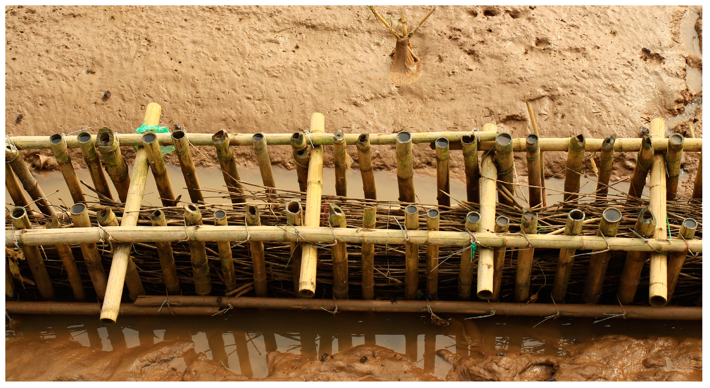
Brushwood fences have been applied as an alternative porous supportive structure for mangrove restoration along the Mekong Delta coast. By using mainly natural materials, i.e., bamboo and tree branches, fences are considered as a nature-based solution for the protection of shorelines and mangrove forests. This low-cost structure has become more convenient for application on the extremely gentle coast of the Mekong Delta, whereas solid structures were intensively expensive and technically challenging. Installed in front of the mangrove belt to dissipate wave-current energy, the wooden fences in Figure 1 are assembled with a frame and an inner part [1,2,3]. The frame with vertical bamboo poles has the role of damping a small amount of energy, but also keeping the inner part in place, which consists of bamboo and tree branches in a horizontal orientation [1,2,3,4,5,6]. Even though previous studies observed significant wave energy reduction through field measurements [1,2,5] and simulation studies [6], none of the existing studies concludes that either the frame or the inner part played a significant role in wave energy reduction. Albers and Von Lieberman [4] tested the effect of porosity on flow energy based on the configuration of bamboo fences. These authors only presented experimental results on vertical bamboo poles, while the vital role of the inner parts was neglected. Thus, it is reasonable to expect that the inner part attenuates energy more effectively than the frame because the structure of the inner part was highly dense compared to the frame as can be seen in Figure 1.

Many studies about the resistance of array cylinders mimicking vegetation and porous structure have been carried out by applying drag force. In general, the drag force on an array of cylinders is used to achieve the quantitative wave-current energy for a similar structure. The drag coefficient theoretically and empirically expresses the resistance of an array of cylinders, mimicking vegetation. The typical procedure for quantifying the drag coefficient analytically is to employ the Morison equation for drag force on circular cylinders, as described in [7,8,9]. Additionally, the drag coefficient is often derived experimentally due to the high complexity of the flow-pole interaction [10].

However, for an aggregate of cylinders with irregular diameters, i.e., the inner part (Figure 1), the drag coefficient is challenging to obtain theoretically due to the complexity of the analytical process. In particular, the complex flow conditions inside the structure, including laminar and turbulent conditions, are often unpredictable. A feasible way of describing the drag force is to adopt the concept of the volume average [11,12], resulting in a type of body force in the form of hydraulic gradient I. The hydraulic gradient induced by the drag force was applied by Darcy [13] for viscous flow ($I=au$) and Forchheimer [14] for both viscous and turbulent flow ($I=au+b{u}^2$), where $u$ ($\mathrm{m}/\mathrm{s}$) is flow velocity, $a$ ($\mathrm{s}/\mathrm{m}$) and $b$ (${\mathrm{s}}^2/{\mathrm{m}}^2$) are commonly known to be the friction terms of the whole body of porous structure [15,16].

For many years, the Darcy–Forchheimer equation has been commonly applied for porous structures made of granular material, e.g., gravel, coarse sand, or fine sand. This equation has been applied for permeable beds of spherical particles [17,18,19,20], packed column with granular materials [15,20], and porous rock structures [16,21,22]. For the inner part of the wooden fence, in particular, bamboo and tree branches with an irregular diameter ranging from 1.0 to 2.0 cm are not completely smooth and straight, leading to high porosity and wide-open spaces between the branches. The Darcy–Forchheimer equation is practically suited to obtaining both drag coefficient and friction factors to obtain friction terms of the inhomogeneous arrangement of cylinders.

In the literature, the characteristics of the material are usually influenced by the drag and the Forchheimer coefficient of porous structures or wooden fences, which include the mean diameter of the material, the density, porosity of the structure, and the distance between cylinders. Additionally, the specific surface area—the total fluid–solid contact area of porous media—is an important parameter commonly applied in physics and chemistry in order to determine the effectiveness of filters [23]. The effects of porosity and specific surface area on the wave energy damping of a vertical cylinder array are described in [24], suggesting that greater specific surface area led to greater wave dissipation.

In this study, the values of the constants in the flow resistance equations that can be used to determine the wave damping potential of brushwood fences at both small and large scale were determined. To achieve this goal, experiments were conducted in which a constant flow was forced through the fence material and characterized in terms of the drag coefficient and the Forchheimer friction coefficient. Several hypotheses are posed and tested: (1) the bulk drag coefficient ($\overline{C_D}$) and friction terms are influenced by the flow regime, represented by the Reynolds number; (2) the drag coefficient decreases with increasing porosity, strongly depending on the type of fence arrangements; (3) the Forchheimer coefficients can be linked to the drag coefficient by means of a parameter under high-turbulence conditions.

The contents are presented in five sections. Section 1 is the introduction. The methodology, which provides descriptions of the formula of resistances, the experiment, and the wooden fences, is presented in Section 2. Section 3 and Section 4 present the experimental results and discussion, respectively. Finally, Section 5 presents the conclusions of this study.

2. Methodology

2.1. Formula of Resistances

The drag coefficient of an immersed cylinder array can be used to derive the drag force on an array of cylinders [25]:

$$F_D=\frac{1}{2}\rho DN\overline{C_D}{u}^2\left(N/{\mathrm{m}}^3\right)$$

(1)

where $D$ (m) and $N \left({\mathrm{m}}^{-2}\right)$ are the diameter and the number of cylinders per volume of a porous media, respectively; $u$ (m/s) is the flow velocity, and $\rho$ ($\mathrm{kg}/{\mathrm{m}}^3$) is the fluid density. The bulk drag coefficient ($\overline{C_D}$) is affected by the cylinder characteristic, such as roughness, cross-sectional shape, flow turbulence and cylinder arrangement, and is a function of cylinder density [26,27]. The bulk drag coefficient is also affected by flow regimes around the cylinder depending on Reynolds number ($Re=uD/\nu$, with $\nu$ (${\mathrm{m}}^2/\mathrm{s}$) is the kinematic viscosity).

For a single cylinder, the flow is laminar until $Re\approx 200$, even though the laminar vortexes appear relatively early at $Re\approx 40$ [28]. However, at $Re>200$, the vortices transition to turbulence when the wakes become unstable. Schewe [29] measured a reduction of the drag coefficient ($C_D$) of a circular cylinder repetitious from 100 to 1 associated with the increase of $Re$, up to ${10}^3$. In this stage, the vortexes are generated from laminar conditions at $Re<40$ [28] to turbulent conditions at $Re>200$, causing a rapid decrease of $C_D$. The $C_D$ value is practically constant at around 1.2 at ${10}^4<Re<{10}^5$. Within a cylinder array, the vortex shedding starts at $Re$ from 150 to 200 [26], which might start late, similarly to an isolated cylinder when the porosity of the array increases, leading to a high drag coefficient at this flow stage.

The bulk drag coefficient of array cylinders is also influenced by the wake of the upstream cylinder [30,31] and by the distance and position between neighbouring cylinders [32]. These phenomena are important for randomly arranged cylinders (inhomogeneous arrangement), because spacing and distance are randomly related. When the upstream flow reaches the front cylinders, a velocity reduction in the wake is caused at the downstream cylinder, resulting in a high value of $C_D$. Under high turbulence conditions, the wake is completely turbulent, resulting in the occurrence of a vortex that influences the rear cylinder, and also leading to a lower pressure on the downstream cylinders [32,33]. Depending on the streamwise spacing ($s$) between cylinders, the vortex at the upstream cylinder may cover the downstream cylinder. For example, a single vortex covers the downstream cylinder when $s/D<1.0$, while two vortices appear when $3.0\le s/D<6.0$ [34]. Thus, the value of $C_D$ can be set at the nearest to the upstream neighbor when $s/D<1.0$, with the strongest wake or vortex interaction [26], while the value of $C_D$ decreases when $s/D>3.0$ [26,30].

In principle, porous media resistance forces can be separated into two types, which are the frictional and pressure forces from drag, and the surface friction of individual elements. For a wooden fence with a high Reynolds number flow, it is assumed that the cylinder roughness is small enough to neglect the friction forces; then the pressure forces are only from drag forces ($F_D$), and become the main resistance forces. In this case, the Darcy–Forchheimer equation is applicable, and it includes linear and non-linear forces due to the effects of laminar and turbulent friction, respectively:

$$F_D=a\rho u+b\rho \left|u\right|u$$

(2)

where $a$ ($\mathrm{s}/\mathrm{m}$) and $b$ (${\mathrm{s}}^2/{\mathrm{m}}^2$) are the friction factors, which represent viscosity and turbulence dominance, respectively. These factors are related to the porosity ($n$), the cylinder diameter and the viscosity ($v$) for a steady-state flow, given as [15,16,21]:

$$a=\alpha \frac{{\left(1-n\right)}^2}{n^3}\frac{\nu }{g{D}^2}$$

(3)

$$b=\beta \frac{1-n}{n^3}\frac{1}{gD}$$

(4)

where $\alpha$ and $\beta$ are the dimensionless parameters representing friction terms, which are assumed to change with the geometry of the wooden fence, including bamboo characteristics. The specific surface are—the total fluid–solid contact area of the objects in a porous medium—is sometimes also used to describe the flow resistance (e.g., Arnaud [24]). The specific surface scales with D, and it can be seen above that the laminar and turbulent friction terms have a $SS{A}^2$ and $SSA$ dependency, respectively.

From here, two options are available that can describe the fence resistances, i.e., the dimensional friction factor $a$ and $b,$ or the drag coefficient $C_D$; their relationship is presented in Section 3 (Experimental Results). Here, the hydraulic gradient of the incompressible fluid over a fence thickness [13] is applied to obtain the drag force:

$$I=-\frac{1}{g\rho }\frac{\delta p}{\delta x}$$

(5)

where $I$ is the pressure gradient generated from pressure difference, $\delta p$ ($\mathrm{kg}.{\mathrm{m}}^{-1}{\mathrm{s}}^{-2}$), over the fence thickness, $\delta x$ (m). From here, two expressions of drag force can be found, combining Equations (1) and (2) with Equation (5):

$$I=\frac{DN\overline{C_D}{u}^2}{2g}$$

(6)

$$I=au+b\left|u\right|u$$

(7)

2.2. Experiment Description

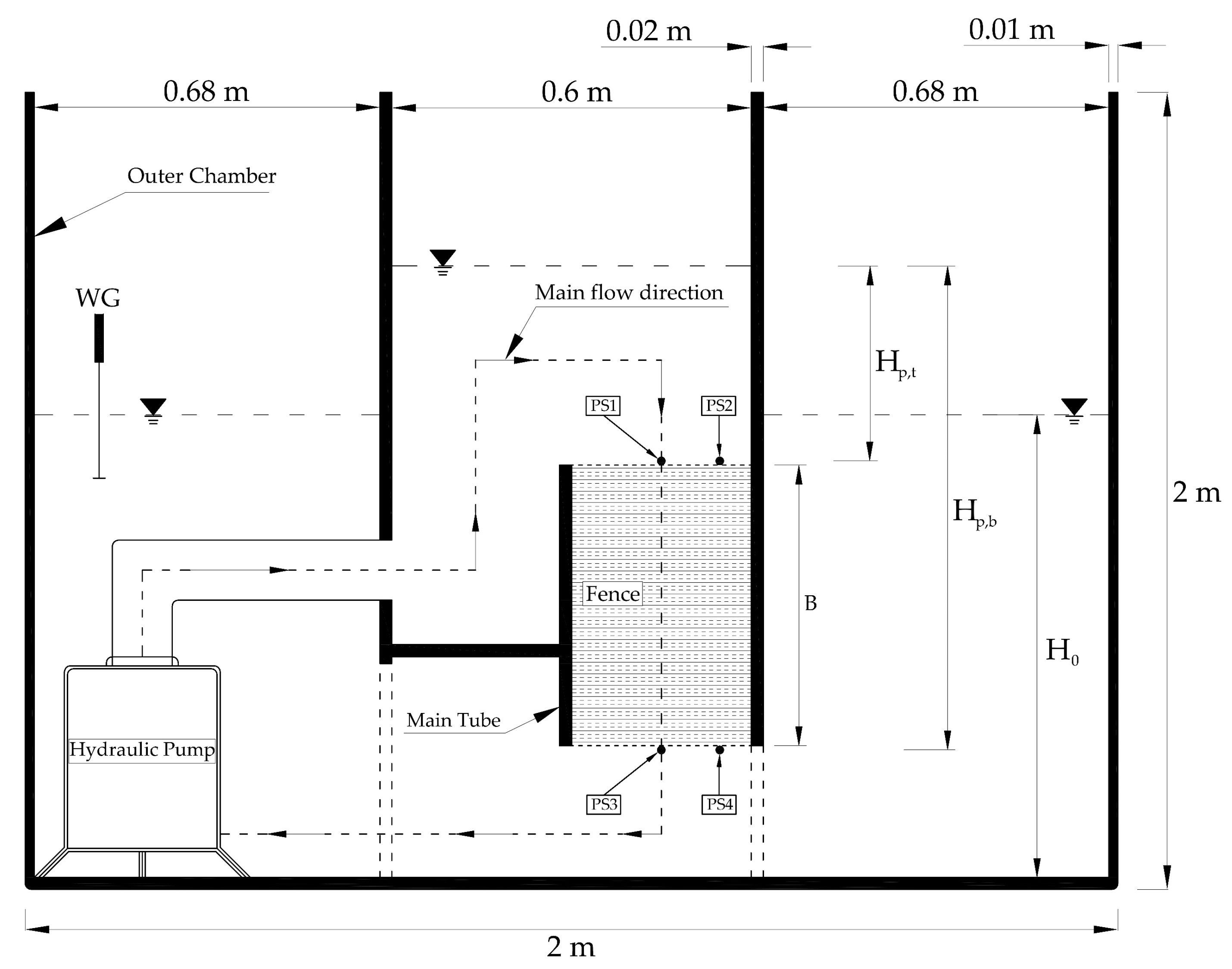
The hydraulic gradient experiments were carried out in the Hydraulic Engineering Laboratory at the Delft University of Technology. The bamboo fence was installed inside a square tube with a cross-sectional area A$\left(26\mathrm{cm}\times 26\mathrm{cm}\right)$ that was placed inside the outer chamber (Figure 2). A hydraulic pump provided a constant flow discharge ($Q\left[\mathrm{m}/{\mathrm{s}}^3\right]$) through the fence with a thickness ($B$), indicated as a dashed line in Figure 2. The hydraulic pump forced the discharge to the open space near the main tube before moving into the fence. The water level was kept above the fence in order to avoid direct pressure on the fence material and to avoid air bubbles inside the pressure sensors (Figure 2). Four pressure sensors (with a range of up to 5 PSI) were used to measure pressure head at the top ($H_{p,t}$, pressure sensors PS1 and PS2) and pressure head at the bottom ($H_{p,b},$pressure sensors PS3 and PS4) of the fence. The difference in pressure head between the top and bottom of the fence can subsequently be estimated by $\Delta H_p=\left|H_{p,b}-H_{p,t}\right|$. The Water level Gauges (WGs) were installed to measure the initial water level outside the main tube ($H_o$) ranging from 0.95 to 1.0 m. This water level was to create the submerged condition for up to the largest thickness of the wooden fence, which was relative to the basin floor for every test.

Fence samples with several thicknesses were tested in each series of flow discharges (see

Table 1. The uncertainty related to measurements during tests.

Q (m3/s)	${\mathit{H}}_0\left(\mathbf{m}\right)$	${\mathit{H}}_{\mathit{p},1}\left(\mathbf{m}\right)$	${\mathit{H}}_{\mathit{p},2}\left(\mathbf{m}\right)$	${\mathit{H}}_{\mathit{p},3}\left(\mathbf{m}\right)$	${\mathit{H}}_{\mathit{p},4}\left(\mathbf{m}\right)$
0.00	$0.98\pm {2.10}^{-2}$	$8.1{10}^{-2}\pm {4.10}^{-3}$	$7.7{10}^{-2}\pm {6.10}^{-3}$	$0.63\pm {2.10}^{-2}$	$0.63\pm {6.10}^{-3}$
${23.10}^{-3}$	$0.96\pm 1.5$	$0.58\pm {2.10}^{-2}$	$0.57\pm {3.10}^{-2}$	$0.65\pm {4.10}^{-2}$	$0.65\pm {2.10}^{-2}$

). The tested thicknesses in Table 1 were chosen from the smallest ($B$ = 0.30 m) to the largest ($B$ = 0.60 m), depending on the material’s thicknesses and based on a minimum thickness of fences in the field corresponding to 0.60 m [1,2]. When the fence samples were set, a set of discharge ($Q$) ranging from $3\times {10}^{-3}$ to $26\times {10}^{-3}$ ${\mathrm{m}}^3/\mathrm{s}$ was imposed through the material. Those discharge quantities were selected based on the expected flow velocities of waves at real fences, on the order of 0.05 to 2.5 m/s. The discharge per total unit area (pores plus solids), or Darcy velocity ($u$ (m/s)) and the pore-flow velocity ($u_n$ (m/s), where $n$ indicates the porosity) were considered to be the characteristic velocities inside porous media [22,35]. These are calculated as

$$u=\frac{Q}{A};u_n=\frac{u}{n}$$

(8)

where A (${\mathrm{m}}^2$) is the cross-sectional area. Hereafter, a fixed discharge was maintained until a steady $H_p$ was reached. The output of all PSs and WGs was recorded in voltage with a sampling frequency of 100 Hz, which could be converted into the corresponding hydraulic heads ($H_p$) by means of linear regression relations. The pressure loss over the fence thickness was derived as

$$I_{*}=\frac{\Delta H_p}{B}$$

(9)

where the subscript “*” indicates each case described in the next section.

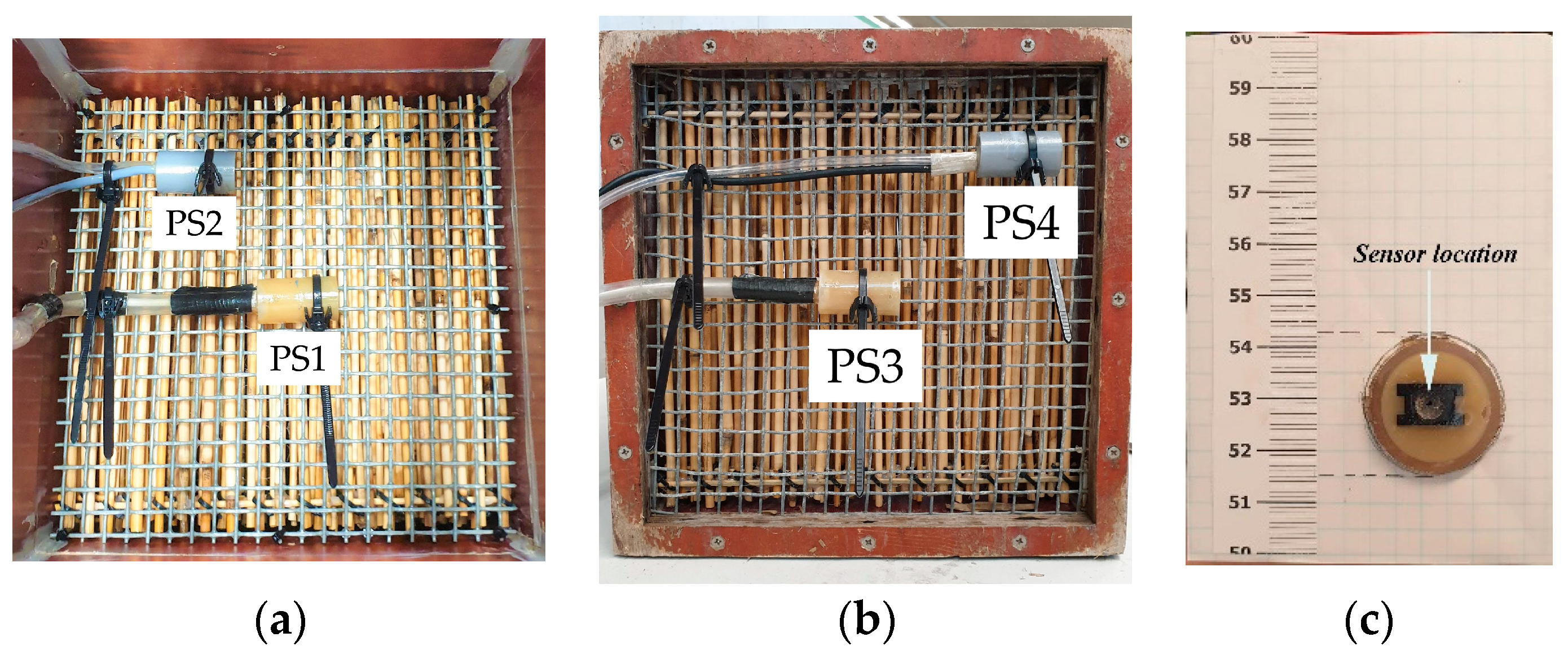
In Figure 3, the fence materials were kept in place by two steel meshes with a thickness of 1.0 mm and with one opening per 1.0 cm. To investigate the effect of steel meshes on the measured pressure heads during the experiment, two steel meshes were installed inside the tube without the bamboo fence. Consequently, the different pressure head ($\Delta H_p$) is similar to one of the tests without the meshes and bamboo fence. Therefore, the effects of two steel meshes could be neglected during the tests. Additionally, all pressure devices had been waterproofed by their manufacturer with the exception of the sensors in the centre of the device (Figure 3c). When pressure sensors were under water, small bubbles were created by the difference in pressure between atmosphere and the water at the entrance of a pressure sensor (Figure 3c), causing extra pressures in the recorded data. By injecting water to fill up the entrance, the pressure sensor could record the required water pressure. This step was only done once for PS3 and PS4 after water surface reached the initial level ($H_0$), because these devices were always underwater. However, this step was repeated each time the fence thickness was changed for both PS1 and PS2.

The uncertainties related to water level and pressure head measurements were calculated as $\pm {\sigma }_{*}$, where $\sigma$ is the standard deviation and the subscript “*” denotes the specific measurements. Table 1 presents the uncertainty of these measurements in two selected flow discharges, Q = 0.0 and Q = 23 ×${10}^{-3} {\mathrm{m}}^3/\mathrm{s}$, for the greatest thickness in each case. It should be noted that the uncertainty of each measurement could be calculated in a time series of data. The output of flow discharge was recorded as a voltage, which was converted into ${\mathrm{m}}^3/\mathrm{s}$ on the basis of linear regression relations. The calibration of flow discharge was done once before tests were started.

For the two discharges included in Table 1, the uncertainty in the production of measured pressure head and the water level outside the main tube was acceptable. Additionally, it should be noted that the water level outside decreased because the flow was kept inside the main tube by the fences at high flow discharge.

2.3. Wooden Fence Descriptions

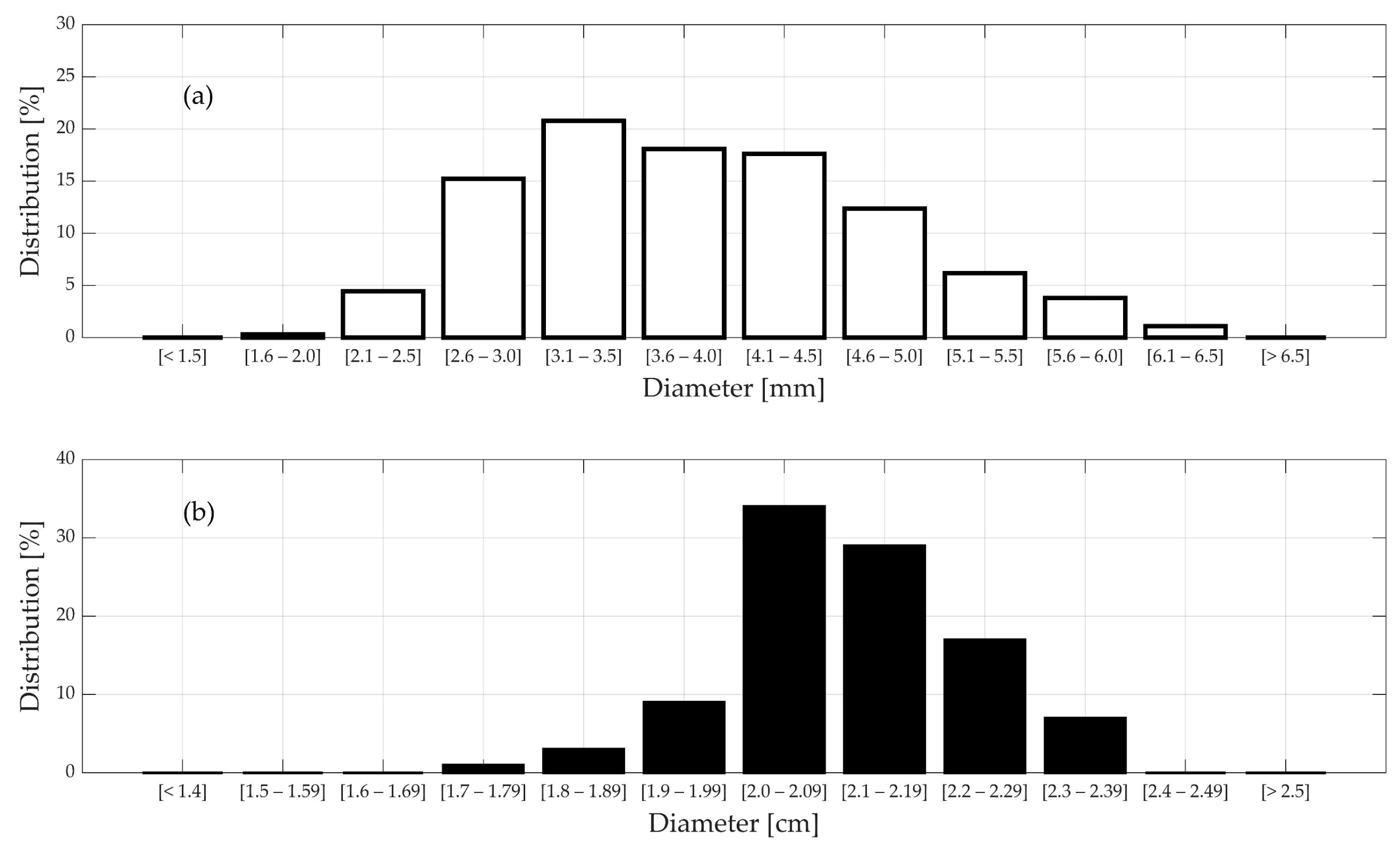
In this study, bamboo poles with a diameter of about 0.02 m were chosen as a large-scale model based on the real fences in the field. The model-scale diameter was chosen by applying a length scale of 5.0 ($L_s=D_p/D_m$), which was available from the supplier. To compare the resistance of small- and real-scale brushwood fences, two sizes of model brushwood were tested using stiff plants, bamboo piles and reeds. Bamboo piles with a mean diameter of 2.1 cm were modelled in real scale, while bamboo reeds of 4.0 mm diameter were employed for small-scale modelling. These natural materials were used as they have natural variations in diameter and length between branches. The small-scale brushwood, used in a wave model with irregular waves, was used to determine possible scale effects. Bamboo diameters were chosen from a statistical analysis of 630 samples with the small diameter and 100 samples for the larger diameter, representing the model and full scale (prototype), respectively. In Figure 4, model diameters are shown to have a wide range of diameters from 2.6 to 4.5 mm in two thirds of the total samples (Figure 4a), while the majority of the prototype diameters range from 2.1 to 2.3 cm in half of the total samples (Figure 4b). The mean diameter, $D_m$ of 4.0 mm and $D_p$ of 2.1 cm, was chosen to characterize the brushwood diameter. The subscripts “m” and “p” refer to the model and the prototype, respectively.

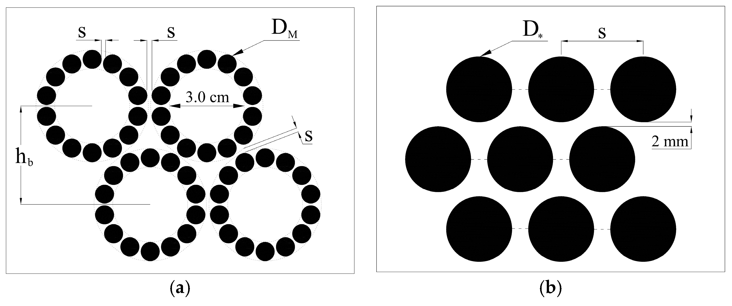
Illustrations of inhomogeneous and staggered configurations are presented in Figure 5. While the inhomogeneous arrangement is indicated to be a regular arrangement in Figure 5a, the diameter and the spanwise spacing had a random character in the experiment. With respect to the inhomogeneous arrangements, mats formed by parallel bamboo reeds connected by steel wire were rolled around a ring in order to generate a large spacing similar to tree branches in the field (Figure 5a), while each case of staggered arrangements contains several reeds per layer (Figure 5b). Specifically, 14 bamboo sticks of diameter $D_m$ were rolled around a 3.0-cm-diameter ring and connected by steel cables in the inhomogeneous case, resulting in an outer diameter of each branch of about 3.5 cm. The distance between each branch ($h_b$) was about 3.0 cm. For the staggered arrangement, case 2 and case 3 contained 20 and 34 sticks of $D_m$ per layer, respectively. Case 4 and case 5 contained 04 and 08 piles of $D_p$ per layer, respectively. The ratio $s/D$ of every configuration corresponds to the smallest distance that generates the highest turbulence conditions. It should be noted that a smaller $s/D$ leads to higher density. However, there is a similar $s/D$ between case 1 and 3, resulting in a different porosity. This difference is caused by the vertical spacing of case 1 ($h_b$ = 3.0 cm), which is significantly larger than case 3 (roughly 3 mm).

In addition to the $s/D$, the specific surface area (SSA) can influence the process of porous flow and the adsorption capacity through/of wooden fences. The SSA factor can be calculated by the ratio of the solid interface area to bulk volume of a wooden fence [36]:

$$SSA=\frac{\pi DNL}{Bulk volume}\left[{\mathrm{m}}^2/{\mathrm{m}}^3\right]$$

(10)

where L is the bamboo length, which is equal to 1.0 m, and the bulk volume is 1.0 ${\mathrm{m}}^3$. The results of density, porosity, SSA, and $s_{*}/D$, where the subscript “*” is indicated for each case, are presented in

Table 2. Samples of bamboo fences in experiments.

Case	Sample	Arrangement SSA (1/m)	D (mm)	Thicknesses B (cm)	Density (Sticks/m2)	$\mathit{n}$	${\mathit{s}}_{*}/\mathit{D}(-)$
Case 1		Inhomogeneous SSA = 100.8	4.00	26.5 34.5 39.0 45.5 58.0	8011	0.90	1.00
Case 2		Staggered SSA = 107.5	4.00	25.5 33.0 42.0 53.5	8547	0.89	1.25
Case 3		Staggered SSA = 164.5	4.00	29.0 39.5 47.0 54.5	13,077	0.80	1.00
Case 4		Staggered SSA = 38.1	20.0	26.5 36.5 46.0	603	0.80	1.36
Case 5		Staggered SSA = 76.2	20.0	26.5 36.5 46.0	1207	0.62	0.23

.

3. Experimental Results

Firstly, the relationship between the pressure gradient and the Darcy velocity was investigated. The pressure gradient was determined as the ratio of the hydraulic head loss to the fence thickness $B$. Then, the effect of Reynolds number on the mean flow drag coefficient was derived.

3.1. Observation of Pressure Gradient

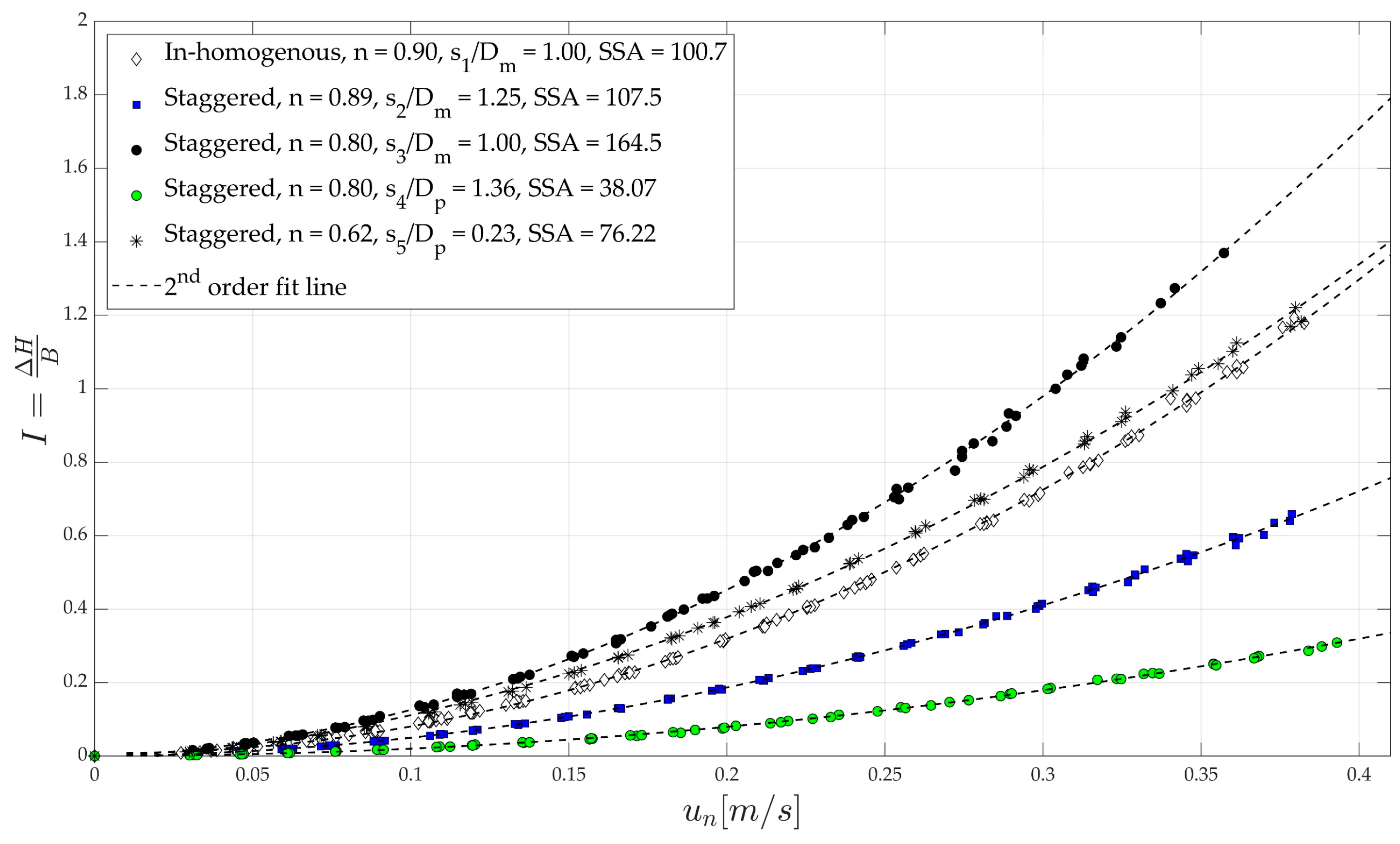
For flow through a porous medium, pressure losses can be represented by the summation of the contribution of laminar flow and turbulent flow, which are proportional to the velocity ($u$) and the quadratic velocity ($u^2$), respectively [15,16]. Figure 6 presents the relationship between the pressure gradient ($I=\Delta H/B$) and the velocity ($u$) for all cases. The Darcy–Forchheimer term in Equation (7), $au+b{u}^2$, is a 2nd-order polynomial fit observed at all states of flow.

As can be observed in Figure 6, the hydraulic gradients ($I$) increase with the increase of velocity in every case. At low velocity, $u$ < 0.05 m/s, all of the hydraulic gradients are similar due to the viscosity effect. However, the hydraulic gradient starts to increase quickly when $u$ > 0.05 m/s, and the quantity of $I_{*}$, again, with the subscript “*” denoting cases 1 to 5, is different between each case. The differences in $I$ between each case increase with increasing velocity, which is to be expected for the quadratic law, due to the different minimum spacing, $s_{*}/D_m$ and $s_{*}/D_p$. For the same porosity of 80%, $I_3$ (black circles) and $I_4$ (green circles) are observed to have a large difference. This is the result of the higher capacity of absorption through the $SS{A}_4$ of 38.07 ($s_4/D_p$ of 1.36) than $SS{A}_3$ of 164.5 ($s_3/D_m$ of 1.00). Additionally, in Figure 6, the decrease of $s/D$ leads to larger differences of $I$ during the increase of velocity, especially at the highest velocity. For example, $I_5$ (black asterisks) is larger than $I_2$ (blue squares), corresponding to larger $s_2/D_m$ than $s_5/D_p$. However, there is an exception for inhomogeneous cases (white diamonds). Even though the spacing $s_1/D_m$ is relatively larger than $s_5/D_p$ (Table 1), $I_1$ is slightly similar to $I_5$ (black asterisks). The explanation is that the local $u$ of case 5 is much higher than the local $u$ in case 1, but the energy loss of case 1, which is proportional to $u^2$, is roughly faster than the energy loss in case 5. In particular, the permeability of case 1 increases due to the large space inside each branch, leading to great energy loss as a result of the thickness. However, the specific surface area of case 5 leads to a similar energy loss to that in case 1.

If the hydraulic gradient is divided by $u^2$, the ratio $I/u^2$ will represent the turbulence contribution to the flow resistance. If this ratio is constant for varying $u$, the viscosity contribution to flow resistance is negligible. The relationship of the ratio $I/u^2$ and the velocity ($u$) is presented in Figure 7. It is shown that the viscosity contribution at the low velocity ($u<0.1$ m/s) occurs for most of the small-scale cases, while the turbulence contribution for large-scale cases appears at every stage of the flow. For example, $I/u^2$ decreases slightly in cases 2 (blue squares) and 4 (green circles) at the highest velocity, while the $I/u^2$ value starts to decrease at velocity $u$ > 0.1 m/s in case 1 (white diamonds). The turbulence effects might occur even later in case 3 (black circles) and case 5 (black asterisks).

3.2. Effect of Reynolds Number on Bulk Drag Coefficient

The effect of the flow regime, represented by the influence of Reynolds number ($R{e}_n=uD/n\nu$) on the bulk drag coefficient ($\overline{C_D}$), is obtained from Equation (6) as

$$\overline{C_D}=\frac{2gI}{DN{u}_n^2}$$

(11)

where the hydraulic gradient $I$ ($\mathrm{kg}/\mathrm{m}$), gravity acceleration $g$ ($\mathrm{m}/{\mathrm{s}}^2$), pore flow velocity $u_n$ (m/s) and fence characteristics depend on the number of cylinders per ${\mathrm{m}}^2$ and bamboo diameter $D$ [m].

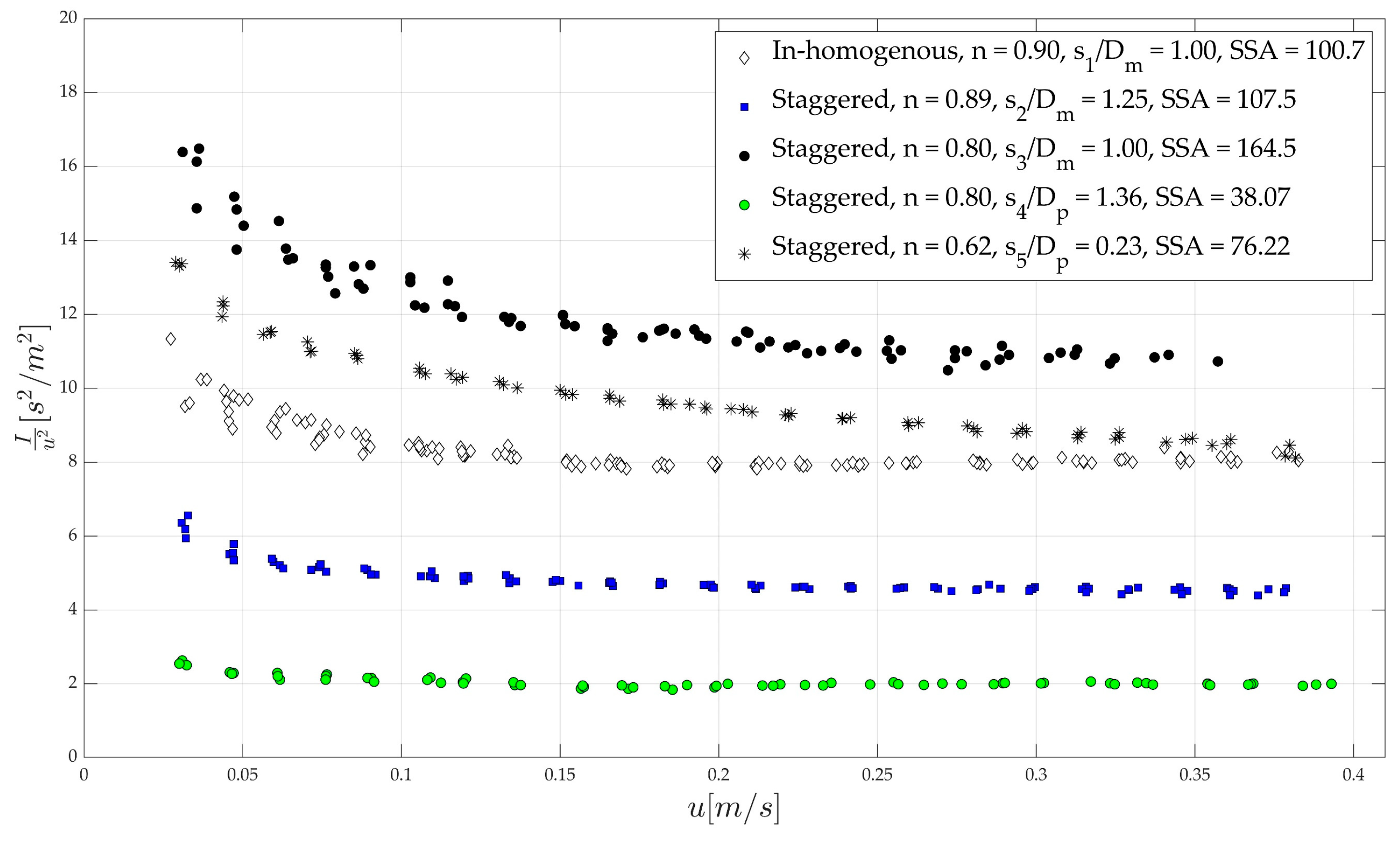
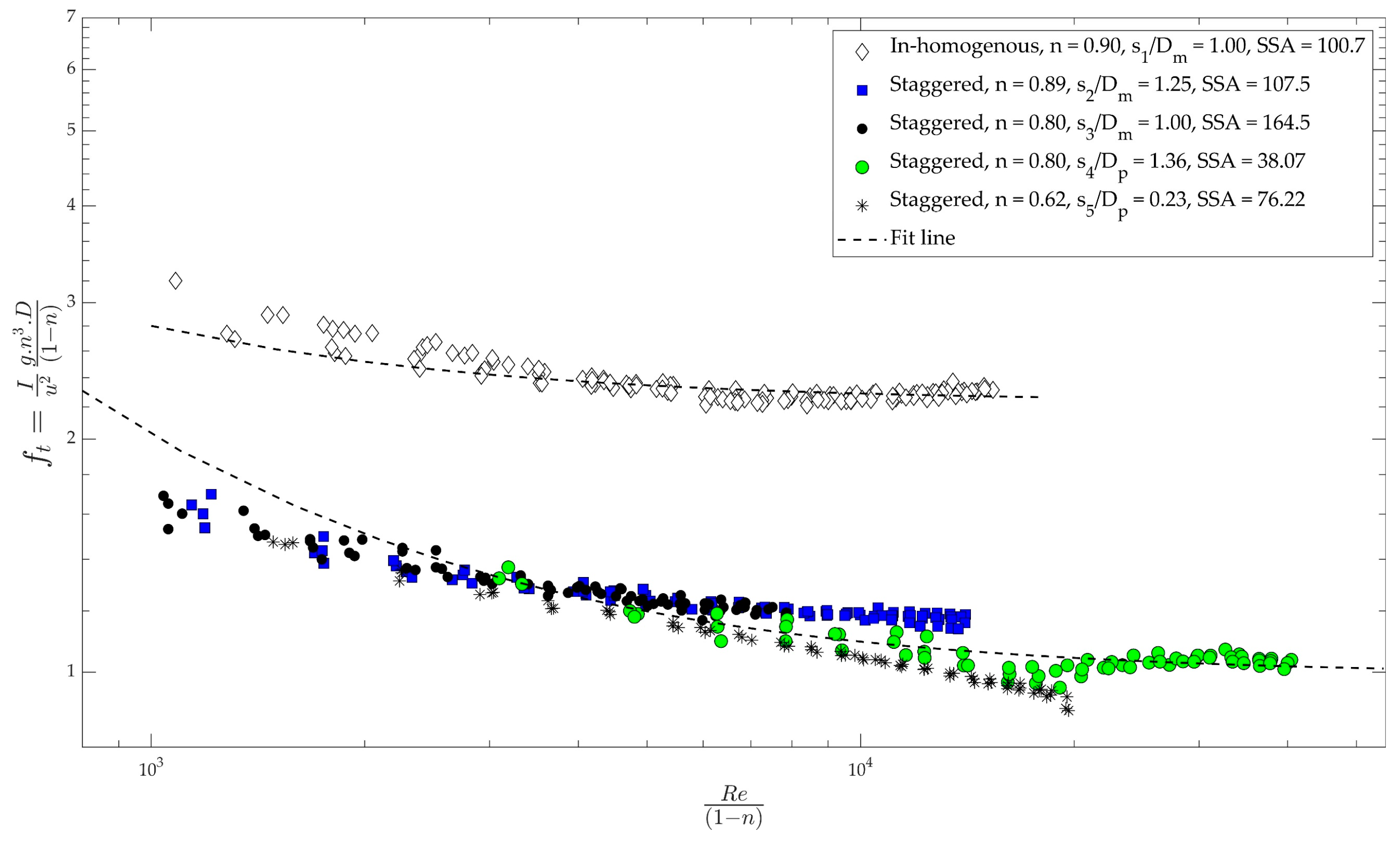
Figure 8 shows the relationship between the bulk drag coefficient and Reynolds number. As can be observed from Figure 8, at $R{e}_n\approx 150$ the wake of all upstream cylinders causes a decrease in velocity at the downstream cylinders, resulting in a high value of $\overline{C_D}$ of 3.0–6.0 related to the model cases (blue squares, white diamonds and black circles), while $\overline{C_D}$ is 2.5–4.0 in the prototype cases (green circles and black asterisks) at $R{e}_n \approx 1000$. For the model cases, $\overline{C_D}$ gradually decreases with increasing $R{e}_n\approx 150-1000$ (under turbulent conditions). For example, $\overline{C_D}$ decreases to 3.87, 2.0, and 1.99 for cases 1, 2 and 3, respectively. For full-scale cases, $\overline{C_D}$ decreases to nearly 1.98 and 0.9 at $R{e}_n>1000$ for cases 4 and 5, respectively. Moreover, $\overline{C_D}$ of cases 3 and 4 is overlapping at $R{e}_n>1000,$ due to a similar porosity of 80%, even though pressure gradients differ greatly between them (Figure 6). It should be noted that $\overline{C_D}$ depends on fence characteristics, e.g., $D$, porosity and arrangements. Thus, the hydraulic behaviour of the flow inside the two cases might be similar.

For a large Reynolds number ($Re \ge$ 150), $\overline{C_D}$ becomes nearly constant, and is a function of fence characteristics, except for case 5. $\overline{C_D}$ decreases due to the increase of incoming velocity through the narrow entrance between cylinders that generates the vortex oscillation of upstream cylinders. For case 1 to case 4, the downstream cylinders are affected within the vortex streets of the upstream cylinders resulting in high $\overline{C_D}$. However, $\overline{C_D}$ of case 5 is relatively small at high Reynolds numbers, which is reflected by its having the strongest vortex interactions at the upstream cylinders. Moreover, $\overline{C_D}$ between the various cases is/are different, which can be explained by the ratio $s/D$. Lower $s/D$ leads to a higher $\overline{C_D}$. This trend occurs both in the full-scale cases (4 and 5) and in the model cases (2 and 3). For example, $\overline{C_{D,4}}$ (1.98) is higher than $\overline{C_{D,5}}$ (0.92) due to the greater ratio of $s_4/D_p$ (1.35) than $s_3/D_p$ (0.23) (see Table 2). Moreover, $\overline{C_{D,2}}$ and $\overline{C_{D,3}}$ have a similar value of 2.0, even though $s/D$ is different, with values of 1.25 and 1.0, respectively. Interestingly, the inhomogeneous arrangement exhibits the highest $\overline{C_D}$ value. This may be due to the more widely spaced branches, reducing the shielding effect of upstream branches, as is confirmed by Nepf [26]. Moreover, an explanation for this phenomenon is an extra reduction when the upstream flow goes through the upstream bamboo reeds and reaches the wide space branches.

In this study, the formulation of the power regression between $\overline{C_D}$ and $R{e}_n$ determined the best fit to be $R^2>0.88$. The formulation is separated into inhomogeneous (case 1), staggered with 89% porosity (case 2), staggered with 80% porosity (cases 3, 4), and staggered with 62% porosity (case 5), as presented in

Table 3. $\overline{C_D}$and$R{e}_n$ relation formulas.

Formula	$\mathbf{Best}\mathbf{Fit}\left({\mathit{R}}^2\right)$	Arrangement	n	$\mathit{s}/\mathit{D}$	Legend
$\overline{C_{D,1}}=3.87+{\left(\frac{177.2}{R{e}_n}\right)}^{1.23}$	0.88	Inhomogeneous; Model	0.90	1.00	This study
$\overline{C_{D,2}}=2.00+{\left(\frac{121.2}{R{e}_n}\right)}^{1.05}$	0.96	Staggered; Model	0.89	1.25	This study
$\overline{C_{D,3}}=1.99+{\left(\frac{326}{R{e}_n}\right)}^{0.65}$	0.96	Staggered; Model	0.80	1.00	This study
$\overline{C_{D,4}}=1.98+{\left(\frac{586}{R{e}_n}\right)}^{1.39}$	0.84	Staggered; Prototype	0.80	1.36	This study
$\overline{C_{D,5}}=0.92+{\left(\frac{65536}{R{e}_n}\right)}^{0.25}$	0.99	Staggered; Prototype	0.62	0.23	This study
$\overline{C_D}=2.10+{\left(\frac{793}{R{e}_n}\right)}^{2.39}$	0.72	Staggered; Model	0.96	unknown	[9]
$\overline{C_D}=1.04+{\left(\frac{730}{R{e}_n}\right)}^{1.37}$	0.89	Staggered; Model	0.96	unknown	[10]

.

Figure 8 also describes a comparison of the relationship between $\overline{C_D}$ and $R{e}_n$ to/with the previous studies, i.e., the authors of [9,10] found the formula of $\overline{C_D}$ relating to $R{e}_n,$ from experimental results of wave and current interaction with vegetation. It can be shown from the results of all cases that the $\overline{C_D}$ value follows the same pattern of decreasing at relatively low $R{e}_n$ and becomes nearly stable at relatively high $R{e}_n$. In Figure 8, the $\overline{C_D}$ of all is relatively higher than that found in [10], whereas the $C_D$ of cases 2, 3, and 4 are very similar to the value found in [9] at Re_n > 1000. This difference could be due to characteristics that are uniquely different between fences and vegetation. The narrow distances between cylinders of wooden fences ($s/D$) were below 1.3, and this is lower than that of 3.0 [10] and 4.7 [9]. As mentioned, the vortex formation around the upstream cylinder less effectively influenced the downstream one when $s/D$ was larger than 3.0, causing a decrease of $C_D$ values [26,30]. Additionally, the $C_D$ under wave conditions increased as a result of the effects of vortex formation from the upstream and downstream cylinders in a wave cycle that was found in both previous studies [9,10]. When a steady current was involved, the vortices shifted to the downstream side, resulting in a decrease of $C_D$ [10].

3.3. Forchheimer Coefficient of Fences

As mentioned in the previous section, the pressure gradient ($I$) is related to the quadratic of Darcy velocity ($u^2$) at most flow rates (Figure 6). It should be noted that stationary flows were applied to every test. Therefore, the turbulence effect could play a major role in the resistance of wooden fences in comparison to the viscosity effect. This means that the linear term ($a\left|u\right|$) in the Forchheimer equation, as shown in Equation (7), can be neglected, yielding $I=bu\left|u\right|$. The expression of coefficient $b$ is included in parameter $\beta$, which should be constant.

From Equations (3), (4), and (7), the full Forchheimer equation is yielded as follows:

$$I=\alpha \frac{{\left(1-n\right)}^2}{n^3}\frac{v}{g{D}^2}u+\beta \frac{\left(1-n\right)}{n^3}\frac{1}{gD}{u}^2$$

(12)

Next, two new forms of Equation (12) can be expressed:

$$\frac{I}{u}\frac{g{D}^2{n}^3}{v{\left(1-n\right)}^2}=\alpha +\beta \frac{uD}{\left(1-n\right)v}=f_v$$

(13)

$$\frac{I}{u^2}\frac{gD{n}^3}{\left(1-n\right)}=\alpha {\left[\frac{uD}{\left(1-n\right)v}\right]}^{-1}+\beta =f_t$$

(14)

The left sides of Equations (13) and (14) are the ratio of pressure losses to the viscous term (viscosity friction, $f_v$) and the turbulence term (turbulent friction, $f_t$).

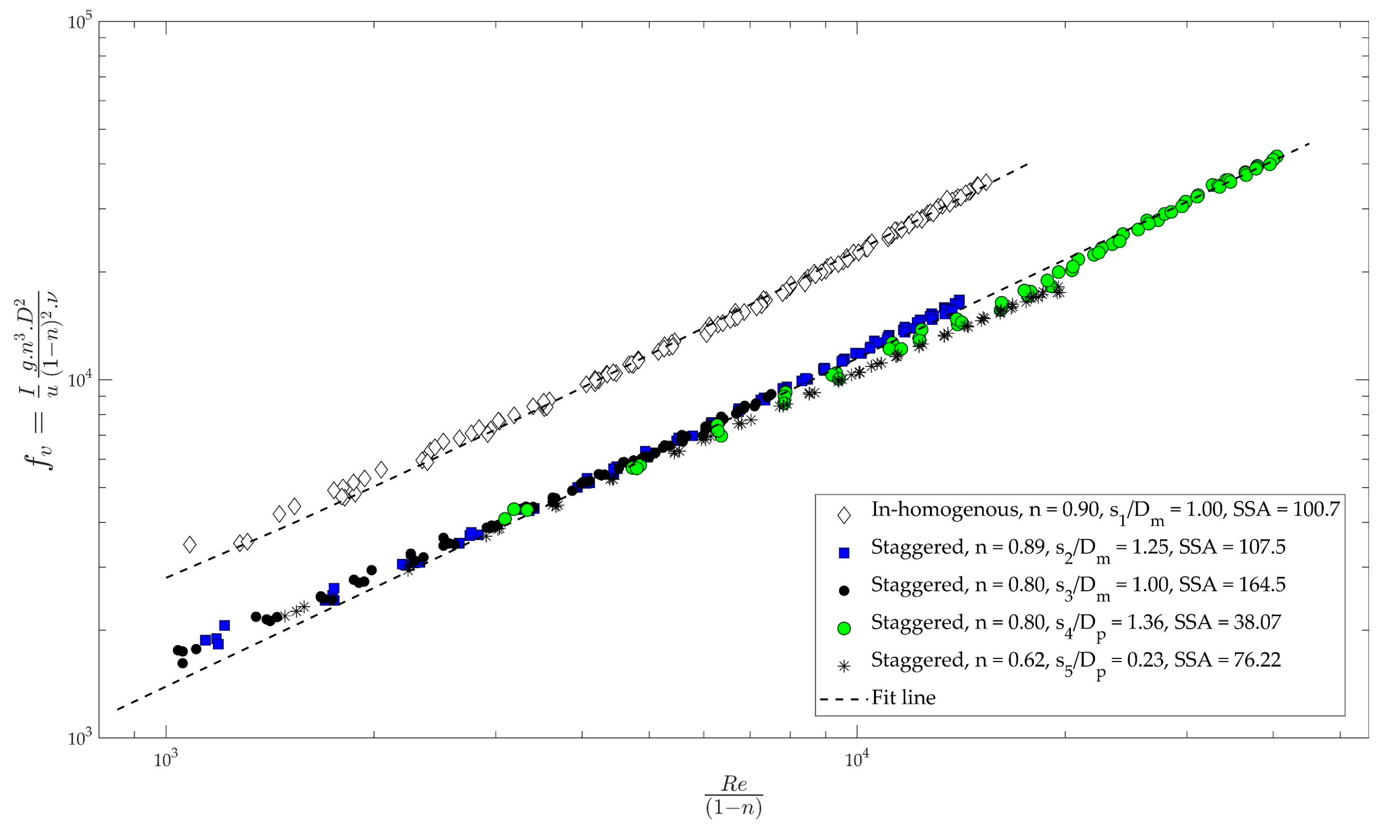
The dimensionless coefficients $\alpha$ and $\beta$ for each case were obtained from the linear relation between $f_v$ and $Re/\left(1-n\right)$ supporting in Figure 9, with a coefficient of determination of over 90%. The $\alpha$ and $\beta$ values of each case are also presented in

Table 4. $\alpha$ and $\beta$ value from linear relation between $f_v$ and $Re/\left(1-n\right)$.

Case	D (mm)	n	${\mathit{\alpha }}_{ *}$	${\mathit{\beta }}_{ *}$	$\mathit{\alpha }$	$\mathit{\beta }$	$\overline{{\mathit{C}}_{\mathit{D}}}$
1	4.0	0.90	566.6	2.234	566.6	2.234	3.89
2	4.0	0.89	569.7	1.128	978.1	0.912	1.98
3	4.0	0.80	580.9	1.125			2.20
4	20.0	0.80	516.3	1.016			1.99
5	20.0	0.62	1444	0.872			0.92

The subscript “*” is denoted for each case.

. The experimental results presented in Table 4 show the dependency of the $\beta$ value on the porosity of the fence. The lower the porosity, the lower the $\beta$ value. For example, $\beta$ from 1.02 to 1.13 corresponds to $n$ = 0.8 and 0.9, while this value is 0.87 at $n$ = 0.62 for the same staggered arrangements. However, there is an exception in the case with a similar porosity, illustrated by case 1 ($n$ = 0.90, $\beta$ = 2.23, SSA = 100.7) and case 2 ($n$ = 0.89, $\beta$ = 1.13, SSA = 107.5), where the $\beta$ value of case 1 is about two times larger than case 2, which can be explained by the difference of cylinder configuration.

In Figure 10, the power relation between $f_t,$ representing the $\beta$ value and $Re/\left(1-n\right),$ is similar to the power plot between $\overline{C_D}$ and $R{e}_n$. As can be seen, the turbulent friction of/in inhomogeneous cases, i.e., $f_v$ = 2.0, is higher than in the staggered cases, $f_t$ = 1.0 at $Re$ > 1000. This relationship is also more convergent than the relationship of $\overline{C_D}$, as shown in Figure 8, especially for all staggered cases.

4. Discussion

4.1. Pressure Loss between Fence Thicknesses

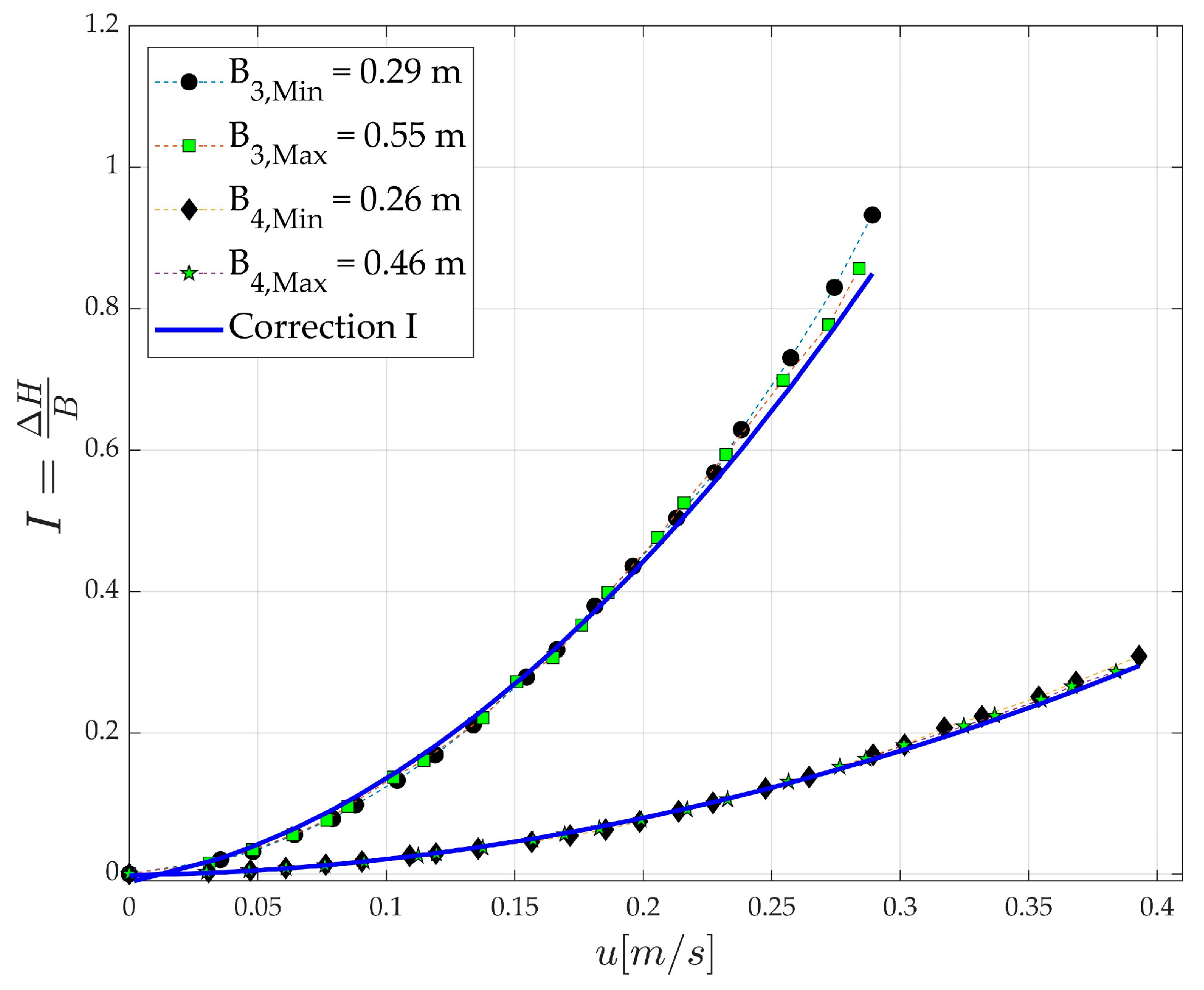
It is hypothesized that hydraulic gradients of all thicknesses were quantitively similar for the same cases. However, an extra pressure loss at the in- and out-flow, especially at high flow rates, might occur when the thickness was increased from thin to thick. The extra pressure loss can be explained by the increase of possible obstructions, leading to flow reduction at the in- and out-flow entrance. However, the extra pressure loss was not easy to obtain from measurements. Therefore, the correction of I between the thinnest and thickest fences should be dealt with using the following formula:

$$I=\frac{\Delta H_2-\Delta H_1}{B_2-B_1}$$

(15)

where the subscript “1” and “2” represent thinner and thicker thicknesses, respectively. It should be noted that other parameters, such as wall effects, wall friction, and extra thicknesses from steel meshes, could influence the measured signals. Fortunately, these effects play a minor role in a different pressure loss between two thicknesses. Comparison of I between two fence thicknesses and the correction I of cases 3 and 4 are plotted against velocity in Figure 11. For case 3, the hydraulic gradient I of two thicknesses was higher than the correction I at u > 0.2 m/s. This trend might be caused by the increase of obstruction and possibly random diameter of small-scale bamboo reeds when thicknesses were changed. Interestingly, the correction I and hydraulic gradient of case 4 were closely matched. One possible explanation for this is the stable flow condition at the in- and out-flow entrance.

4.2. Effects of Specific Surface Area

The specific surface area (SSA), the total fluid–solid contact area of the wooden fence, is proportional to the diameter of the bamboo cylinders. In Table 2, SSA also increases with the decrease of both porosity and $s/D$, except for inhomogeneous cases. Forchheimer parameters might be based on the specific surface area, which is dependent on the characteristics of the wooden fence, i.e., bamboo diameter and porosity. The laminar and turbulent friction terms have $SS{A}^2$ and $SSA$ dependency, as described in Equations (13) and (14), respectively. The value the laminar and turbulent friction terms is inversely proportional to the order of the SSA magnitudes. The friction terms of cases with lower SSA, i.e., case 2 (blue square, SSA = 107.5) and case 4 (green circle, SSA = 38.1), are greater than the high SSA cases in the same scale (see Figure 9 and Figure 10). However, the high friction of inhomogeneous cases was caused by the extra magnitude of both laminar and turbulent friction due to the wide space inside each branch. Additionally, the laminar drag or friction might cause extra flow reduction even if the flow is in turbulent condition.

For the bulk drag coefficient, the laminar drag caused high flow reduction, resulting in a decrease in the value of $\overline{C_D}$ with the increase of flow rate. Additionally, the phenomena associated with $\overline{C_D}$, i.e., the wake and vortex oscillation of array cylinders, became greater in proportion to SSA, leading to higher values of $\overline{C_D}$ compared to existing studies. However, SSA was less influenced by turbulent drags when $R{e}_n$ > 150 for the model cases. In particular, the values of $\overline{C_D}$ for cases 2 and 3 were similar at 2.0, even when SSA significantly increased from 107.5 to 164.5. For large-scale cases, the SSA effect might still influence the laminar drag at high $R{e}_n$, especially in case 4 with a high SSA = 76.2.

4.3. The Link between Drag Coefficients and Forchheimer Parameter

The experimental results also point out two relationships between resistance factors, the drags ($\overline{C_D}$), and the turbulent friction ($\beta$) coefficients throughout the two different methods. In particular, the expression of these coefficients can be emphasized by the vortex of upstream cylinders increasing the velocity reduction after each layer of branches and mats under high-turbulence conditions. However, according to Equation (14), $\beta$ values are more related to flow over solid volume ($Re/(1-n$)) than $\overline{C_D}$ values, which are dependent on flows over porous volume ($Re/n$). This theory can be supported by Figure 7 and Figure 9, when the $\beta$ values of all staggered cases were more convergent into a fitted line of power than $\overline{C_D}$. Thus, there should be a link between friction and bulk drag coefficients, because both coefficients were linearly related to a quadratic component of flow velocity. Hereafter, the link between these two coefficients can be described as:

$$\beta =\frac{2n}{\pi }\overline{C_D}$$

(16)

This link is obtained from combining Equations (11) and (12). It is noted that porosity is $n=1-N\pi D^2/4$. This relationship strongly depends on the porosity of a fence, and can be applied to cylinders, as presented in Table 4.

Moreover, Ergun [15] applied the law of fluid flow through packed columns with small particle materials to introduce the viscosity and kinetic energy losses corresponding Equations (13) and (14) in this study. In Ergun’s study, the values for parameters ${\alpha }_E$ and ${\beta }_E$, with the subscript “E” used for Ergun’s study, were 150 and 1.75, respectively. Comparing these parameters in Table 4, ${\alpha }_E$ was much smaller than all tested cases due to high laminar friction at the low flow rate. Interestingly, ${\beta }_E$ was larger than most of the staggered cases, while it was smaller than the inhomogeneous case. It can be explained that the fence characteristics exert an influence on both in terms of viscosity and turbulent energy loss. For case 1, the wide space inside each branch could cause a velocity reduction from upstream and downstream cylinders resulting in an additional energy loss into both the friction factors $a$ and $b$. In contrast, most of the staggered cases have a narrow space between cylinders, leading to lower friction compared to Ergun’s study. Additionally, the specific surface area in Ergun’s study might have less effect on laminar and turbulent friction than this study due to different material characteristics.

5. Conclusions

The resistance of a brushwood fence was investigated by determining the hydraulic gradient over a fence sample under stationary flow. Fence samples were installed in both a model- and a full-scale setup with inhomogeneous and staggered configurations with porosities varying from 62% to about 90%. Based on the experiment results, the $\overline{C_D}$ was strongly dependent on the fence’s porosity, the minimum spacing ratio ($s/D$) configuration, and the Reynolds number. With decreasing $\overline{C_D}$ values, $R{e}_n$ increased from 150 to 1000 and became stable at $R{e}_n$ > 1000. The $\overline{C_D}$ value also decreased when the ratio $s/D$ was reduced in all full-scale tests. This ratio can be linked directly to the fence’s porosity, which supports the result indicating that the lowest porosity case has the smallest $\overline{C_D}$.

Moreover, the application of Forchheimer’s law and Ergun’s equation resulted in a new method for predicting the bulk drag coefficient of wooden fences in the field. Specifically, the inner parts of a wooden fence in the field also have an inhomogeneous arrangement [1,2,3,4,5,6], usually causing the space between bamboo branches to be irregular. It is reasonable for the flow reduction to be somewhat unpredictable. The specific surface area can explain the resistance of wooden fences, which is dependent on diameter and porosity. Greater SSA leads to higher laminar drag, which causes higher Cd at the low Re. The decrease of SSA also leads to an increase in both the laminar and turbulent friction of wooden fences. Our findings for $\overline{C_D}$ and $\beta$ of inhomogeneous cases may predict this coefficient in the field. The link between $\overline{C_D}$ and the Forchheimer coefficient $\beta$ for a high Reynolds flow was determined to be $\overline{C_D}=\beta \pi /2n$.

References

- Schmitt, K.; Albers, T.; Pham, T.T.; Dinh, S.C. Site-specific and integrated adaptation to climate change in the coastal mangrove zone of Soc Trang Province, Viet Nam. J. Coast. Conserv. 2013, 17, 545–558. [Google Scholar] [CrossRef] [Green Version]
- Albers, T.; San, D.C.; Schmitt, K. Shoreline Management Guidelines: Coastal Protection in the Lower Mekong Delta. Dtsch. Ges. Für Int. Zs. (GiZ) GmbH Manag. Nat. Resour. Coast. Zone Soc Trang Prov 2013, 1, 1–124. [Google Scholar]
- Schmitt, K.; Albers, T. Area Coastal Protection and the Use of Bamboo Breakwaters in the Mekong Delta; Elsevier Inc.: Amsterdam, The Netherlands, 2014. [Google Scholar] [CrossRef]
- Albers, T.; Von Lieberman, N. Current and Erosion Modelling Survey. Dtsch. Ges. Für Int. Zs. (GiZ) GmbH Manag. Nat. Resour. Coast. Zone Soc Trang Prov. 2011, 1, 1–61. [Google Scholar]
- Van Cuong, C.; Brown, S.; To, H.H.; Hockings, M. Using Melaleuca fences as soft coastal engineering for mangrove restoration in Kien Giang, Vietnam. Ecol. Eng. 2015, 81, 256–265. [Google Scholar] [CrossRef]
- Dao, T.; Stive, M.J.F.; Hofland, B.; Mai, T. Wave Damping due to Wooden Fences along Mangrove Coasts. J. Coast. Res. 2018, 34, 1317–1327. [Google Scholar] [CrossRef]
- Anderson, M.E.; Smith, J.M. Wave attenuation by flexible, idealized salt marsh vegetation. Coast. Eng. 2014, 83, 82–92. [Google Scholar] [CrossRef]
- Mendez, F.J.; Losada, I.J. An empirical model to estimate the propagation of random breaking and nonbreaking waves over vegetation fields. Coast. Eng. 2004, 51, 103–118. [Google Scholar] [CrossRef]
- Ozeren, Y.; Wren, D.G.; Wu, W. Experimental investigation of wave attenuation through model and live vegetation. J. Waterw. Port Coast. Ocean Eng. 2013, 140, 4014019. [Google Scholar] [CrossRef]
- Hu, Z.; Suzuki, T.; Zitman, T.; Uittewaal, W.; Stive, M. Laboratory study on wave dissipation by vegetation in combined current–wave flow. Coast. Eng. 2014, 88, 131–142. [Google Scholar] [CrossRef]
- Hsu, T.-J.; Sakakiyama, T.; Liu, P.L.-F. A numerical model for wave motions and turbulence flows in front of a composite breakwater. Coast. Eng. 2002, 46, 25–50. [Google Scholar] [CrossRef]
- Liu, P.L.-F.; Lin, P.; Chang, K.-A.; Sakakiyama, T. Numerical modeling of wave interaction with porous structures. J. Waterw. Port Coast. Ocean Eng. 1999, 125, 322–330. [Google Scholar] [CrossRef]
- Darcy, H.P.G. Les Fontaines Publiques de la Ville de Dijon. Exposition et Application des Principes à Suivre et des Formules à Employer dans les Questions de Distribution d’eau, etc; Victor Dalmont: Paris, France, 1856. [Google Scholar]
- Forchheimer, P. Wasserbewegung durch boden. Z. Ver. Deutsch Ing. 1901, 45, 1782–1788. [Google Scholar]
- Ergun, S. Fluid flow through packed columns. Chem. Eng. Prog. 1952, 48, 89–94. [Google Scholar]
- Van Gent, M.R.A. Wave interaction with permeable coastal structures. Int. J. Rock Mech. Min. Sci. Geomech. Abstr. 1996, 6, 277A. [Google Scholar]
- Rao, P.T.; Chhabra, R.P. Viscous non-Newtonian flow in packed beds: Effects of column walls and particle size distribution. Powder Technol. 1993, 77, 171–176. [Google Scholar] [CrossRef]
- Tiu, C.; Zhou, J.Z.Q.; Nicolae, G.; Fang, T.; Chhabra, R.P. Flow of viscoelastic polymer solutions in mixed beds of particles. Can. J. Chem. Eng. 1997, 75, 843–850. [Google Scholar] [CrossRef]
- Machač, I.; Cakl, J.; Comiti, J.; Sabiri, N.E. Flow of non-Newtonian fluids through fixed beds of particles: Comparison of two models. Chem. Eng. Process. Process. Intensif. 1998, 37, 169–176. [Google Scholar] [CrossRef]
- De Castro, A.R.; Radilla, G. Non-Darcian flow of shear-thinning fluids through packed beads: Experiments and predictions using Forchheimer’s law and Ergun’s equation. Adv. Water Resour. 2017, 100, 35–47. [Google Scholar] [CrossRef] [Green Version]
- Van Gent, M.R.A. Stationary and oscillatory flow through coarse porous media. In Communications on Hydraulic and Geotechnical Engineering, No. 1993-09; TU Delft: Delft, The Nertherlands, 1993. [Google Scholar]
- Jensen, B.; Gjøl, N.; Damgaard, E. Investigations on the porous media equations and resistance coef fi cients for coastal structures. Coast. Eng. 2014, 84, 56–72. [Google Scholar] [CrossRef]
- Kantzas, A.; Bryan, J.; Taheri, S. Fundamentals of fluid flow in porous media. Pore Size Distrib. 2012, 1, 1–336. [Google Scholar]
- Arnaud, G.; Rey, V.; Touboul, J.; Sous, D.; Molin, B.; Gouaud, F. Wave propagation through dense vertical cylinder arrays: Interference process and specific surface effects on damping. Appl. Ocean Res. 2017, 65, 229–237. [Google Scholar] [CrossRef]
- Dalrymple, R.A.; Kirby, J.T.; Hwang, P.A. Wave diffraction due to areas of energy dissipation. J. Waterw. Port Coast. Ocean Eng. 1984, 110, 67–79. [Google Scholar] [CrossRef]
- Nepf, H.M. Drag, turbulence, and diffusion in flow through emergent vegetation. Water Resour. Res. 1999, 35, 479–489. [Google Scholar] [CrossRef]
- Sumer, B.M. Hydrodynamics around Cylindrical Strucures; World Scientific: Singapore, 2006. [Google Scholar]
- Williamson, C.H.K. The natural and forced formation of spot-like ‘vortex dislocations’ in the transition of a wake. J. Fluid Mech. 1992, 243, 393–441. [Google Scholar] [CrossRef]
- Schewe, G. On the force fluctuations acting on a circular cylinder in crossflow from subcritical up to transcritical Reynolds numbers. J. Fluid Mech. 1983, 133, 265–285. [Google Scholar] [CrossRef]
- Bokaian, A.; Geoola, F. Wake-induced galloping of two interfering circular cylinders. J. Fluid Mech. 1984, 146, 383–415. [Google Scholar] [CrossRef]
- Blevins, R.D.; Scanlan, R.H. Flow-Induced Vibration. J. Appl. Mech. 1977, 44, 802. [Google Scholar] [CrossRef]
- Luo, S.C.; Gan, T.L.; Chew, Y.T. Uniform flow past one (or two in tandem) finite length circular cylinder (s). J. Wind. Eng. Ind. Aerodyn. 1996, 59, 69–93. [Google Scholar] [CrossRef]
- Žukauskas, A. Heat transfer from tubes in crossflow. In Advances in Heat Transfer; Elsevier: Amsterdam, The Netherlands, 1972; pp. 93–160. [Google Scholar]
- Zdravkovich, M.M. Review of flow interference between two circular cylinders in various arrangements. J. Fluids Eng. 1977, 99, 618–633. [Google Scholar] [CrossRef]
- Burcharth, H.F.; Andersen, O.K. On the one-dimensional steady and unsteady porous flow equations. Coast. Eng. 1995, 24, 233–257. [Google Scholar] [CrossRef]
- Tosco, T.; Marchisio, D.L.; Lince, F.; Sethi, R. Extension of the Darcy–Forchheimer law for shear-thinning fluids and validation via pore-scale flow simulations. Transp. Porous Media 2013, 96, 1–20. [Google Scholar] [CrossRef]
Figure 1.
Wooden fences in the field [6]. The construction includes the frame (two rows of 6–8 cm diameter bamboo poles) and the inner part (a bunch of branches of 1–2 cm diameter bamboo reeds). Reproduced with permission from Dao et al. (2018), Journal of Coastal Research; published by BioOne, 2018.
Figure 2.
Experimental setup. The outer chamber covers the main tube, inside of which fences are installed. During a test, a constant flow discharge, provided by the hydraulic pump, goes through the fence. The different pressures measured by the pressure sensors (PS) are given as .
Figure 3.
Pressure sensors installed at the top (a) and the bottom (b) of the main tube, and the configuration of the pressure head (c).
Figure 4.
Bamboo diameter distribution for (a) model scale and (b) prototype.
Figure 5.
The configurations of wooden fence used in this study: inhomogeneous arrangement (a), and staggered arrangement (b). The “*” denotes the model and the real scale, and , respectively.
Figure 6.
Pressure gradient () plots against pore velocity () of all cases.
Figure 7.
The relation between and .
Figure 8.
Relationship between Reynolds number () and the bulk of drag coefficient ().
Figure 9.
Relationship between and .
Figure 10.
Figure 11.
Comparison of I between two thickness for case 3 and 4, n = 0.80.