Extending the Convergence Domain of Methods of Linear Interpolation for the Solution of Nonlinear Equations

Abstract

Solving equations in abstract spaces is important since many problems from diverse disciplines require it. The solutions of these equations cannot be obtained in a form closed. That difficulty forces us to develop ever improving iterative methods. In this paper we improve the applicability of such methods. Our technique is very general and can be used to expand the applicability of other methods. We use two methods of linear interpolation namely the Secant as well as the Kurchatov method. The investigation of Kurchatov’s method is done under rather strict conditions. In this work, using the majorant principle of Kantorovich and our new idea of the restricted convergence domain, we present an improved semilocal convergence of these methods. We determine the quadratical order of convergence of the Kurchatov method and order $\frac{1+\sqrt{5}}{2}$ for the Secant method. We find improved a priori and a posteriori estimations of the method’s error.

1. Introduction

We consider solving equation

$$F\left(x\right)=0$$

(1)

using iterative methods. Here $F:\Omega \subset B_1\to B_2$, $B_1,B_2$ are Banach spaces, $\Omega$ is an open region of $B_1$.

Secant method

$$x_{n+1}=x_n-{[x_n,x_{n-1};F]}^{-1}F\left(x_n\right),n=0,1,\dots$$

(2)

is a popular device for solving nonlinear equations. It is due to the following: simplicity of the method; small amount of calculations on each iteration and use of the value of an operator from only two previous iterations in the iterative formula of the method. A lot of works are dedicated to this method [1,2,3]. In [4] the Secant method is used for solving the nonlinear least squares problem. The Kurchatov’s method of linear interpolation

$$x_{n+1}=x_n-{[2x_n-x_{n-1},x_{n-1};F]}^{-1}F\left(x_n\right),n=0,1,\dots$$

(3)

is less known. This method has the same order of convergence as Newton’s method but does not require the calculation of derivatives. In (2) and (3), $[u,v;F]$ is a divided difference of the first order for the operator F at the points u and v [5,6].

In this work we will investigate the Secant method and Kurchatov’s method using the Kantorovich’s principle of majorants. For the first time, this principle was used by L.V. Kantorovich for investigating the convergence of the classical and modified Newton’s method, having built for the nonlinear operator a majorizing real quadratic function [7]. Corresponding to this, the iterative sequence for nonlinear operator is majorized by a converging sequence for nonlinear equation with one variable. Later the nonlinear majorants for investigating other methods of solving nonlinear functional equations have been built. In work [8] with the help of the majorant principle, a method with the order of convergence $1.839...$, which in its iterative formula uses the value of an operator from the three previous iterations, is investigated. Specifically, a real cubical polynomial, which majorizes the given nonlinear operator is built. With that, the Lipschitz conditions are put upon the divided differences’ operator of the second order [8,9]. We investigate the Secant method with different conditions that have been put upon the nonlinear operator. In particular, if the Lipschitz condition for the divided differences of the first order are fulfilled, the quadratic majorizing function of one variable is built, and if the Lipschitz condition for operator of divided difference of the second order are fulfilled, the cubical majorizing function is built. The cubical majorizing function for Kurchatov’s method is also built. Methods of linear interpolation applied to these functions produce a numerical sequence, which majorizes by norm the iterative sequence, produced by applying these methods to the nonlinear operator. In all cases, the a priori and a posteriori error estimations of the linear interpolation methods are also provided.

2. Divided Differences and Their Properties

Let us assume that $x,y$ and z are three points in region $\Omega$.

Definition 1

([6]). Let F be a nonlinear operator defined on a subset Ω of a Banach space $B_1$ with values in a Banach space $B_2$ and let $x,y$ be two points of Ω. A linear operator from $B_1$ to $B_2$ which is denoted by $[x,y;F]$ and satisfies the conditions:

(1) for all fixed two points $x,y\in \Omega$

$$[x,y;F](x-y)=F\left(x\right)-F\left(y\right),$$

(4)

(2) if exist a Fréchet derivative $F^{\prime }\left(x\right)$, then

$$[x,x;F]=F^{\prime }\left(x\right)$$

(5)

is called a divided difference of F at the points x and y.

Note that (4) and (5) do not uniquely determine the divided difference with the exception of the case when $B_1$ is one-dimensional. For specific spaces, the differences are defined in Section 6.

Definition 2

([8]). The operator $[x,y,z;F]$ is called divided difference of the second order of function F at the points x, y and z, if

$$[x,y,z;F](y-z)=[x,y;F]-[x,z;F].$$

(6)

We assume that for $[x,y;F]$ and $[x,y,z;F]$ the conditions of the Lipschitz type are being satisfied in the following form:

$$\parallel [x,y;F]-[x,z;F]\parallel \le p\parallel y-z\parallel ,x,y,z\in \Omega ,$$

(7)

$$\parallel [y,x;F]-[z,x;F]\parallel \le \overline{p}\parallel y-z\parallel ,x,y,z\in \Omega ,$$

(8)

$$\parallel [x,y,z;F]-[u,y,z;F]\parallel \le q\parallel x-u\parallel ,u,x,y,z\in \Omega .$$

(9)

If the divided difference $[x,y;F]$ of F satisfies (7) or (8), then F is differentiable by Fréchet on $\Omega$. Moreover, if (7) and (8) are fulfilled, then the Fréchet derivative is continuous by Lipschitz on $\Omega$ with the Lipschitz constant $L=p+\overline{p}$ [8].

Let us denote $U(x_0,\tau )=\{x\in \Omega :\parallel x-x_0\parallel <\tau \}$ and $\overline{U}(x_0,\tau )=\{x\in \Omega :\parallel x-x_0\parallel \le \tau \}$. The semilocal convergence of the Secant method uses the conditions $\left(C\right)$:

$\left(c_1\right)$$F:\Omega \to Y$ is nonlinear operator with $[·,·;F]:\Omega \times \Omega \to$$\mathcal{L}$$(B_1,B_2)$ denoting a first order divided difference on $\Omega$.

$\left(c_2\right)$ Let $x_0,x_{-1}\in \Omega$. Suppose that the linear operator $A_0$ is invertible and let $a,c$ be nonnegative numbers such that

$$\parallel x_0-x_{-1}\parallel \le a,\parallel A_0^{-1}F\left(x_0\right)\parallel \le c.$$

$\left(c_3\right)$ Assume that the following conditions hold on $\Omega$

$$\parallel A_0^{-1}(A_0-[x_0,x_0;F])\parallel \le \tilde{p}\parallel x_0-x_{-1}\parallel \mathrm{for}\mathrm{some}\tilde{p}>0$$

or

$$\parallel A_0^{-1}(A_0-[x_0,x_0;F])\parallel \le b_0.$$

Moreover, assume the following Lipschitz conditions hold for all $u,v,z\in \Omega$ for some ${\tilde{p}}_0>0$ and ${\tilde{\tilde{p}}}_0>0$

$$\parallel A_0^{-1}([x_0,x_0;F]-[x_0,v;F])\parallel \le {\tilde{p}}_0\parallel v-x_0\parallel$$

and

$$\parallel A_0^{-1}([x_0,u;F]-[z,u;F])\parallel \le {\tilde{\tilde{p}}}_0\parallel z-x_0\parallel .$$

Set $b=min\{b_0,\tilde{p}a\}$. Define

$${\Omega }_0=\Omega \cap U(x_0,\tilde{r}),\tilde{r}=\frac{1-b}{{\tilde{p}}_0+{\tilde{\tilde{p}}}_0}$$

provided $b<1.$

$\left(c_4\right)$ The following Lipschitz conditions hold on ${\Omega }_0$ for some ${\overline{p}}_0>0$ and ${\overline{\overline{p}}}_0>0$

$$\parallel A_0^{-1}([z,u;F]-[z,v;F])\parallel \le {\overline{p}}_0\parallel u-v\parallel$$

and

$$\parallel A_0^{-1}([u,z;F]-[v,z;F])\parallel \le {\overline{\overline{p}}}_0\parallel u-v\parallel .$$

Set $p=max\{{\overline{p}}_0,{\overline{\overline{p}}}_0\}.$

$\left(c_5\right)$ Suppose $pa<1$, and define ${\displaystyle \overline{r}=\frac{1-pa}{2p}}$ and

$$\overline{h}\left(t\right)=-p{t}^2+(1-pa)t.$$

Moreover, suppose

$$c\le \overline{h}\left(\overline{r}\right)=\frac{{(1-pa)}^2}{4p}.$$

(10)

$\left(c_6\right)$$U_0=\overline{U}(x_0,{\overline{r}}_0)\subset \Omega$, where ${\overline{r}}_0$ is the unique root in $(0,\overline{r}]$ of equation $\overline{h}\left(t\right)-c=0$.

Remark 1.

The following Lipschitz condition is used in the literature for the study of iterative methods using divided differences [1,2,3,4,8,9,10,11,12,13,14,15,16] for $p_0>0$

$$\parallel A_0^{-1}([x,y;F]-[u,v;F])\parallel \le p_0(\parallel x-u\parallel +\parallel y-v\parallel ),$$

although it is not really needed, since tighter conditions are really needed (see conditions $\left(C\right)$ and proofs that follow).

By these definitions we have

$${\tilde{p}}_0\le p_0,$$

$${\tilde{\tilde{p}}}_0\le p_0,$$

$$p\le p_0,$$

$${\Omega }_0\subseteq \Omega .$$

The sufficient semilocal convergence criterion in the literature arrived at different ways and corresponding to $\left(c_5\right)$ [1] is

$$c\le h\left(r\right)=\frac{{(1-p_{0}a)}^2}{4p_0},$$

(11)

where

$$h\left(t\right)=-p_0{t}^2+(1-p_{0}a)t,r=\frac{1-p_{0}a}{2p_0}$$

provided that $p_{0}a<1$ (stronger than $pa<1$).

Then, we have

$$c\le h\left(r\right)\Rightarrow c\le \overline{h}\left(\overline{r}\right),$$

(12)

but not necessarily vice versa, $r\le \overline{r}$ and $\overline{h}\left(t\right)\le h\left(t\right)$ for each $t\in [0,r]$.

Hence, the applicability of the Secant method is extended and under no additional conditions, since all new Lipschitz conditions are specializations of the old condition. Then, in practice the computation of $p_0$ requires that of of the other $“p”$ as special cases. Some more advantages are reported after Proposition 1. It is also worth noticing that $\left(c_3\right)$ and $\left(c_4\right)$ help define ${\Omega }_0$ through which ${\overline{p}}_0,{\overline{\overline{p}}}_0$ and p are defined too. With the old approach p depends only on $\Omega$, which contains ${\Omega }_0$. In our approach the iterates $x_n$ remain in ${\Omega }_0$ (not $\Omega$ used in [1]). That is why our new p constants are at least as tight as $p_0$. There is where the novelty of our paper lies and the new idea helps us extend the applicability of these methods. It is also worth noticing that the new constants are specializations of the old ones. Hence, no additional conditions are added to obtain these extensions.

It is worth noting from the proof of Theorem 1 that ${\Omega }_0$ can be defined as ${\displaystyle {\Omega }_0=\Omega \cap U\left(x_0,\frac{1-b}{{\tilde{p}}_0}\right)}$ or ${\displaystyle {\Omega }_0=\Omega \cap U\left(x_0,\frac{1-b}{{\tilde{\tilde{p}}}_0}\right)}$.

Theorem 1.

Suppose that the conditions $\left(C\right)$ hold. Then, the iterative procedure (2) is well defined and the sequence generated by it converges to a root $x_{*}$ of the equation $F\left(x\right)=0$. Moreover, the following error estimate holds:

$$\parallel x_n-x_{*}\parallel \le t_n,n=-1,0,1,\dots ,$$

(13)

where

$$t_{-1}={\overline{r}}_0+a,t_0={\overline{r}}_0,$$

(14)

$$t_{n+1}=t_n\frac{p{t}_{n-1}}{1-pa-2p{\overline{r}}_0+p(t_n+t_{n-1})},n=0,1,\dots$$

(15)

The semilocal convergence of the discussed methods was based on the verification of the criterion (11). If this criterion is not satisfied there is no guarantee that the methods converge. We have now replaced (11) by (10) which is weaker (see (12)).

Proof. 

Notice that the sequence ${\left\{t_n\right\}}_{n\ge 0}$ is generated by applying the iterative method (2) to a real polynomial

$$f\left(t\right)=p{t}^2+(1-pa+2p{\overline{r}}_0)t.$$

It is easy to see that the sequence monotonically converges to zero. In addition, we have

$$\begin{array}{ccc}\hfill t_{n+1}-t_{n+2}& =& {\displaystyle {\left(\frac{f\left(t_{n+1}\right)-f\left(t_n\right)}{t_{n+1}-t_n}\right)}^{-1}f\left(t_{n+1}\right)}\hfill \\ \hfill & =& {\displaystyle \frac{p(t_{n-1}-t_{n+1})}{1-pa-p(2t_0-t_n-t_{n+1})}(t_n-t_{n+1}).}\hfill \end{array}$$

(16)

We prove by using of induction that the iterative method is well defined and that

$$\parallel x_n-x_{n+1}\parallel \le t_n-t_{n+1}.$$

(17)

Using $\left(c_2\right),\left(c_5\right)$, (13), (14) and

$$\begin{array}{ccc}\hfill t_0-t_1& =& {\displaystyle \frac{t_{-1}-t_0}{f\left(t_{-1}\right)-f\left(t_0\right)}f\left(t_0\right)}\hfill \\ \hfill & =& {\displaystyle \frac{t_{-1}-t_0}{p(t_{-1}^2-t_0^2)+(1-pa-2p{\overline{r}}_0)(t_{-1}-t_0)}f\left(t_0\right)=f\left({\overline{r}}_0\right)=\overline{h}\left({\overline{r}}_0\right)=c,}\hfill \end{array}$$

(18)

it follows that (17) holds for $n=-1,0$. Let k be a nonnegative integer and for all the $n\le k$ fulfills (17). If $A_{k+1}=[x_{k+1},x_k;F]$, then by $\left(c_3\right)$, we have

$$\begin{array}{ccc}\hfill \parallel I-A_0^{-1}{A}_{k+1}\parallel & =& \parallel A_0^{-1}(A_0-A_{k+1})\parallel \hfill \\ \hfill & =& \parallel A_0^{-1}([x_0,x_{-1};F]-[x_0,x_0;F]+[x_0,x_0;F]-[x_0,x_k;F]+[x_0,x_k;F]-[x_{k+1},x_k;F])\parallel \hfill \\ \hfill & \le & b+{\tilde{p}}_0\parallel x_0-x_k\parallel +{\tilde{\tilde{p}}}_0\parallel x_0-x_{k+1}\parallel \hfill \\ \hfill & \le & b+{\tilde{p}}_0(t_0-t_k)+{\tilde{\tilde{p}}}_0(t_0-t_{k+1})<b+({\tilde{p}}_0+{\tilde{\tilde{p}}}_0)t_0\le b+({\tilde{p}}_0+{\tilde{\tilde{p}}}_0)\overline{r}\hfill \\ \hfill & \le & {\displaystyle b+({\tilde{p}}_0+{\tilde{\tilde{p}}}_0)\frac{1-b}{{\tilde{p}}_0+{\tilde{\tilde{p}}}_0}=1.}\hfill \end{array}$$

(19)

In view of the Banach lemma [7] $A_{k+1}$ is invertible, and

$$\parallel A_{k+1}^{-1}{A}_0\parallel \le (1-pa-p(\parallel x_0-x_{k+1}\parallel +\parallel x_0-x_k{\parallel \left)\right)}^{-1}.$$

(20)

Next, we prove that the iterative method exist for n = k + 1. We get

$$\begin{array}{ccc}\hfill \parallel x_{k+1}-x_{k+2}\parallel & =& \parallel A_{k+1}^{-1}F\left(x_{k+1}\right)\parallel \hfill \\ \hfill & =& \parallel A_{k+1}^{-1}(F\left(x_{k+1}\right)-F\left(x_k\right)-A_k(x_{k+1}-x_k))\parallel \hfill \\ \hfill & \le & \parallel A_{k+1}^{-1}{A}_0\parallel \parallel A_0^{-1}([x_{k+1},x_k;F]-A_k)\parallel \parallel x_k-x_{k+1}\parallel .\hfill \end{array}$$

(21)

By condition $\left(c_4\right)$, we have

$$\begin{array}{ccc}\hfill \parallel A_0^{-1}([x_{k+1},x_k;F]-A_k)\parallel & =& \parallel A_0^{-1}([x_{k+1},x_k;F]-[x_k,x_k;F]+[x_k,x_k;F]-[x_k,x_{k-1};F])\parallel \hfill \\ \hfill & \le & p(\parallel x_k-x_{k+1}\parallel +\parallel x_{k-1}-x_k\parallel ).\hfill \end{array}$$

(22)

Then, it follows from (20)–(22)

$${\displaystyle \parallel x_{k+1}-x_{k+2}\parallel \le \frac{p(\parallel x_k-x_{k+1}\parallel +\parallel x_{k-1}-x_k\parallel )\parallel x_k-x_{k+1}\parallel }{1-pa-p(\parallel x_0-x_{k+1}\parallel +\parallel x_0-x_k\parallel )}.}$$

In view of (16) and (17), we obtain

$$\parallel x_{k+1}-x_{k+2}\parallel \le t_{k+1}-t_{k+2}.$$

Hence, the iterative method is well defined for each n. Hence, it follows that

$$\parallel x_n-x_k\parallel \le t_n-t_k,-1\le n\le k.$$

(23)

Estimate (23) shows that ${\left\{x_n\right\}}_{n\ge 0}$ is a Cauchy sequence in space $B_1$ so, it is converging. Let k tend to infinity in formula (23), then we get (13). It is easy to see that $x_{*}$ is the root of equation $F\left(x\right)=0$, because accordingly to (22), we can write

$$\begin{array}{ccc}\hfill \parallel A_0^{-1}F\left(x_{k+1}\right)\parallel & =& \parallel A_0^{-1}([x_{k+1},x_k;F]-A_k)(x_{k+1}-x_k)\parallel \hfill \\ \hfill & \le & p(\parallel x_k-x_{k+1}\parallel +\parallel x_k-x_{k-1}\parallel )\parallel x_k-x_{k+1}\parallel .\hfill \end{array}$$

(24)

 □

Corollary 1.

The convergence order of iterative Secant method (2) is equal to $\frac{1+\sqrt{5}}{2}$.

Proof. 

From equality (15) it follows that the order of convergence of the real sequence ${\left\{t_n\right\}}_{n\ge 0}$ is the only positive root of the equation $s^2-s-1=0$, i.e., $s^{*}=\frac{1+\sqrt{5}}{2}=1.618\dots$. Given inequality (13), according to Kantorovich’s majorant principle, we obtain that the sequence ${\left\{x_n\right\}}_{n\ge 0}$ also has an order of convergence $\frac{1+\sqrt{5}}{2}$. □

Concerning the uniqueness of the solution, we have the result.

Proposition 1.

Under the conditions $\left(C\right)$ further suppose that for $d>0$

$$\parallel A_0^{-1}(A_0-[x_{*},v;F])\parallel \le d(\parallel x_0-x_{*}\parallel +\parallel x_{-1}-v\parallel )$$

holds for all $u,v\in {\Omega }_1$, where ${\Omega }_1=\Omega \cap U(x_0,\overline{R})$, ${\displaystyle \overline{R}=\frac{1-d(a+{\overline{r}}_0)}{d}}$ and provided $d(a+{\overline{r}}_0)<1$, where $x_{*}$ is a solution of equation $F\left(x\right)=0$. Then, $x_{*}$ is the only solution of equation $F\left(x\right)=0$ in the set ${\Omega }_1$.

Proof. 

Let $M=[x_{*},y_{*};F]$, where $y_{*}\in {\Omega }_1$ and $F\left(y_{*}\right)=0$. Then, we get

$$\parallel A_0^{-1}(A_0-[x_{*},y_{*};F])\parallel \le d(\parallel x_0-x_{*}\parallel +\parallel x_{-1}-y_{*}\parallel )<d({\overline{r}}_0+a+\overline{R})=1,$$

so $x_{*}=y_{*}$ follows from $0=F\left(x_{*}\right)-F\left(y_{*}\right)=[x_{*},y_{*};F](x_{*}-y_{*}).$ □

Remark 2.

The result in Proposition 1 improves the corresponding one in the literature using the old condition, since ${\displaystyle R=\frac{1-p_0}{2p_0}\le \overline{R}}$. Hence, we present a larger ball inside which we guarantee the uniqueness of the solution $x_{*}$.

If, additionally, the second divided difference of function F exists and satisfies the Lipschitz condition with constant q, then the majorizing function for $F\left(x\right)$ is a cubical polynomial. Then, the following theorem holds.

Theorem 2.

Under the $\left(C\right)$ conditions (except $\left(c_5\right)$) further suppose

$\left(h_1\right)$ Let us presume that $pa+q{a}^2\le 1$ and denote

$${\displaystyle s={\left\{{(p+qa)}^2+3q(1-pa-q{a}^2)\right\}}^{1/2},\overline{r}=\frac{1-pa-q{a}^2}{p+qa+s}.}$$

Let h be a real polynomial

$$\overline{h}\left(t\right)=-q{t}^3-(p+qa)t^2+[1-pa-q{a}^2]t.$$

It the following inequality is satisfied

$${\displaystyle c\le \overline{h}\left(\overline{r}\right)=\frac{1}{3}·\frac{p+qa+2s}{1-q{a}^2}{\left(\frac{1-pa-q{a}^2}{p+qa+s}\right)}^2}$$

(25)

and the closed ball $U_0=\overline{U}(x_0,{\overline{r}}_0)\subset \Omega$, where ${\overline{r}}_0\in (0,\overline{r}]$ is the root of equation $\overline{h}\left(t\right)=c(1-q{a}^2)$.

$\left(h_2\right)$

$$\parallel A_0^{-1}([x,y,z;F]-[u,y,z;F])\parallel \le q\parallel x-u\parallel .$$

(26)

$\left(h_3\right)$ Conditions of Propositions 1 hold on ${\Omega }_0$.

Then, the iterative method (2) is well defined and the generated by it sequence converges to the solution $x_{*}$ of the equation $F\left(x\right)=0$. Moreover, the following estimate is satisfied

$$\parallel x_n-x_{*}\parallel \le t_n,n=-1,0,1,2,\dots ,$$

(27)

where

$$t_0={\overline{r}}_0,t_{-1}={\overline{r}}_0+a,$$

(28)

$$a_0=p+3q{\overline{r}}_0+qa,b_0=3q{\overline{r}}_0^2-2a_0{\overline{r}}_0-q{a}^2-pa+1,$$

(29)

$$\begin{array}{c}{\displaystyle t_{n+1}=t_n{t}_{n-1}·\frac{a_0-q(t_n+t_{n-1})}{b_0+a_0(t_n+t_{n-1})-q(t_n^2+t_{n-1}{t}_n+t_{n-1}^2)},}\hfill \\ n=0,1,2,\dots .\hfill \end{array}$$

(30)

This proof is analogous to the proof of Theorem 1.

Remark 3. 

$\left(a\right)$ The majorizing sequences $\left\{t_n\right\}$ are more precise than the one in [1] (using $(p_0,q_0)$ instead of $(p,q)$, respectively).

$\left(b\right)$ Similar advantages we report in the case of Theorem 2, see e.g., [1] where instead of $\left(h_2\right)$ the following condition is used on Ω

$$\parallel A_0^{-1}([x,y,z;F]-[u,y,z;F])\parallel \le q_0\parallel x-u\left|\right).$$

We have

$$q\le q_0$$

(since ${\Omega }_0\subseteq \Omega$).

3. A Posteriori Estimation of Error of the Secant Method

If the constants $a,c,p,q$ are known, then we can compute the sequence ${\left\{x_n\right\}}_{n\ge 0}$ before generating the sequence ${\left\{x_n\right\}}_{n\ge 0}$ by the iterative Secant algorithm. With help of inequalities (13) and (27), the a priori estimation of error of the Secant method is given. We obtain an a posteriori estimation of the method’s error, which is sharper than the a priori one.

Theorem 3.

Let the conditions of the Theorem 2 hold. Denote

$$e_n=p(\parallel x_n-x_{n-1}\parallel +\parallel x_{n-1}-x_{n-2}\parallel )\parallel x_n-x_{n-1}\parallel ,$$

$$g_n=1-pa-2p\parallel x_n-x_0\parallel .$$

Then, the estimate holds for $n=1,2,3,\dots$

$${\displaystyle \parallel x_n-x_{*}\parallel \le \frac{2e_n}{g_n+{(g_n^2-4p{e}_n)}^{\frac{1}{2}}}\le t_n.}$$

Proof. 

By condition $\left(c_4\right)$, we have

$$\begin{array}{ccc}\hfill \parallel I-A_0^{-1}[x_n,x_{*};F]\parallel & =& \parallel A_0^{-1}([x_0,x_{-1};F]-[x_0,x_0;F]+[x_0,x_0;F]\hfill \\ & & -[x_n,x_0;F]+[x_n,x_0;F]-[x_n,x_{*};F])\parallel \hfill \\ & \le & p(\parallel x_0-x_{-1}\parallel +\parallel x_n-x_0\parallel +\parallel x_0-x^{*}\parallel )\hfill \\ & \le & pa+p(2\parallel x_n-x_0\parallel +\parallel x_n-x^{*}\parallel )\hfill \\ & \le & pa+p(2t_0-2t_n+t_n)=pa+2p{t}_0-p{t}_n<pa+2p{t}_0.\hfill \end{array}$$

It is easy to see that $pa+2p{t}_0\le 1$. Then, according to the Banach lemma $[x_n,x_{*};F]$ is invertible, and

$$\begin{array}{ccc}\hfill \parallel {[x_n,x_{*};F]}^{-1}{A}_0\parallel & \le & {\displaystyle \frac{1}{1-p(\parallel x_0-x_{-1}\parallel +\parallel x_n-x_0\parallel +\parallel x_0-x^{*}\parallel )}}\hfill \\ \hfill & \le & (g_n-p\parallel x_n-x_{*}{\parallel )}^{-1}.\hfill \end{array}$$

(31)

From (4) we can write

$$x_n-x_{*}={[x_n,x_{*};F]}^{-1}(F\left(x_n\right)-F\left(x_{*}\right))=\left({[x_n,x_{*};F]}^{-1}{A}_0\right)A_0^{-1}F\left(x_n\right).$$

Using (24) and (31), we obtain an inequality

$$\parallel x_n-x_{*}\parallel \le (g_n-p\parallel x_n-x_{*}{\parallel )}^{-1}{e}_n,$$

from which follows that

$$\begin{array}{ccc}\hfill \parallel x_n-x_{*}\parallel & \le & 2{\{g_n+{(g_n^2-4p{e}_n)}^{\frac{1}{2}}\}}^{-1}{e}_n,\hfill \\ \hfill t_n& =& {\displaystyle \frac{p{t}_n^2+(1-pa-2p{r}_0)t_n}{p{t}_n+(1-pa-2p{r}_0)}}\hfill \\ \hfill & =& {\displaystyle \frac{p(t_{n-2}-t_n)}{1-pa-2p(t_0-t_n)-p{t}_n}(t_{n-1}-t_n)}\hfill \\ \hfill & \ge & {\displaystyle \frac{e_n}{g_n-p\parallel x_n-x_{*}\parallel }\ge \parallel x_n-x_{*}\parallel .}\hfill \end{array}$$

(32)

 □

If the second divided difference of function F exists and satisfies the Lipschitz condition with constant q, then the following theorem holds.

Theorem 4.

Let the conditions of the Theorem 2 hold. Denote

$$e_n=p(\parallel x_n-x_{n-1}\parallel +\parallel x_{n-2}-x_{n-1}\parallel )+q\parallel x_{n-1}-x_{n-2}{\parallel }^2,$$

$$g_n=1-pa-q{a}^2-2p\parallel x_n-x_0\parallel .$$

Then the following estimate holds for $n=1,2,3,...$

$${\displaystyle \parallel x_n-x_{*}\parallel \le \frac{2e_n}{g_n+{(g_n^2-4p{e}_n)}^{\frac{1}{2}}}\le t_n.}$$

Proof. 

The proof of this theorem is similar to the previous theorem, but instead of inequalities (32), the following majorizing inequalities are used

$$\begin{array}{ccc}\hfill t_n& =& {\displaystyle \frac{-q{t}_n^3+a_0{t}_n^2+b_0{t}_n}{-q{t}_n^2+a_0{t}_n+b_0}}\hfill \\ & =& {\displaystyle \frac{p(t_{n-2}-t_n)+q{(t_{n-2}-t_{n-1})}^2+q[2t_0+t_{-1}+t_{n-1}+t_{n-2}+t_n)]}{1-pa-q{a}^2-2p(t_0-t_n)-p{t}_n-(3q{r}_0+qa){(t_0-t_n)}^2-q{t}_n^2-qa{t}_0}}\hfill \\ & \ge & {\displaystyle \frac{p(t_{n-2}-t_n)+q{(t_{n-2}-t_{n-1})}^2}{1-pa-q{a}^2-2p(t_0-t_n)-p{t}_n}\ge \frac{e_n}{g_n-p\parallel x_n-x_{*}\parallel }\ge \parallel x_n-x_{*}\parallel .}\hfill \end{array}$$

 □

4. Semilocal Convergence of the Kurchatov’s Method

Sufficient conditions of semilocal convergence and the speed of convergence of the Kurchatov’s method (3) are determined by the following theorem.

Theorem 5.

Suppose: Conditions $\left(c_1\right)-\left(c_4\right)$, $\left(h_2\right)$ and $\left(h_3\right)$ hold, but with $A_0=[2x_0-x_{-1},x_{-1};F]$ and ${\Omega }_0=\Omega \cap U(x_0,\tilde{r})$, where ${\displaystyle \tilde{r}=\frac{1-\tilde{q}{a}^2}{3{\tilde{p}}_0+{\tilde{\tilde{p}}}_0}}$, provided $\tilde{q}{a}^2<1$ and

$$\parallel A_0^{-1}([2x_0-x_{-1},x_{-1},x_0;F]-[x_0,x_{-1},x_0;F])\parallel \le \tilde{q}\parallel x_0-x_{-1}\parallel .$$

Let us assume that $2q{a}^2\le 1$ and denote

$${\displaystyle s={\left\{{(p+qa)}^2+3q(1-q{a}^2)\right\}}^{1/2},\overline{r}=\frac{1-q{a}^2}{p+qa+s}.}$$

Let $\overline{h}$ be a real polynomial

$$\overline{h}\left(t\right)=-q{t}^3-(p+qa)t^2+(1-q{a}^2)t.$$

Assume

$${\displaystyle c(1-2q{a}^2)\le \overline{h}\left(\overline{r}\right)=\frac{1}{3}·(p+qa+2s){\left(\frac{1-q{a}^2}{p+qa+s}\right)}^2,}$$

$x_0,x_{-1}\in U_0\subseteq V_0=\overline{U}(x_0,3{\overline{r}}_0)\subset \Omega$, and ${\overline{r}}_0\in (0,\overline{r}]$ is the unique root of equation $\overline{h}\left(t\right)-c(1-2q{a}^2)=0$, then the iterative Kurchatov’s method (3) is well defined and the sequence generated by it converges to the solution $x_{*}$ of the equation (1). Moreover, the following inequality is being satisfied

$$\parallel x_n-x_{*}\parallel \le t_n,n=-1,0,1,2,\cdots ,$$

(33)

where

$$t_0={\overline{r}}_0,t_{-1}={\overline{r}}_0+a,$$

$$a_0=p+3q{\overline{r}}_0+qa,b_0=3q{\overline{r}}_0^2-2a_0{\overline{r}}_0-q{a}^2+1,$$

$$\begin{array}{c}{\displaystyle t_{n+1}=t_n·\frac{a_0{t}_n-q{(t_n-t_{n-1})}^2-2q{t}_n^2}{b_0+2a_0{t}_n-q{(t_n-t_{n-1})}^2-3q{t}_n^2},n=0,1,2,\dots }\hfill \end{array}$$

(34)

Proof. 

The proof of the theorem is realized with help of the majorants of Kantorovich. As in Theorem 1 but we also use the crucial estimate

$$\begin{array}{ccc}\hfill \parallel I-A_0^{-1}{A}_{k+1}\parallel & =& \parallel A_0^{-1}(A_0-A_{k+1})\parallel \hfill \\ & =& \parallel A_0^{-1}([2x_0-x_{-1},x_{-1};F]-[x_0,x_{-1};F]+[x_0,x_{-1};F]-[x_0,x_0;F]+[x_0,x_0;F]\hfill \\ & & -[x_{k+1},x_0;F]+[x_{k+1},x_0;F]-[x_{k+1},x_k;F]+[x_{k+1},x_k;F]-[2x_{k+1}-x_k,x_k;F])\parallel \hfill \\ & =& \parallel A_0^{-1}(([2x_0-x_{-1},x_{-1},x_0;F]-[x_0,x_{-1},x_0;F])(x_0-x_{-1})\hfill \\ & & +[x_0,x_0;F]-[x_{k+1},x_0;F]\hfill \\ & & +[x_{k+1},x_0;F]-[x_{k+1},x_k;F]+[x_{k+1},x_k;F]-[2x_{k+1}-x_k,x_k;F])\parallel \hfill \\ & \le & \tilde{q}{a}^2+({\tilde{p}}_0+{\tilde{\tilde{p}}}_0)\parallel x_0-x_{k+1}\parallel +2{\tilde{p}}_0\parallel x_0-x_k\parallel .\hfill \end{array}$$

 □

Corollary 2.

The convergence order of iterative Kurchatov’s procedure (3) is quadratic.

Proof. 

As a result that according to (34) the convergence of the sequence ${\left\{t_n\right\}}_{n\ge 0}$ to zero not higher than quadratic, then there are $C\ge 0$ and $N>0$, that for all $n\ge N$ the inequality holds

$${(t_n-t_{n-1})}^2\le t_{n-1}^2\le C{t}_n.$$

Given this inequality, a quadratic order convergence of the sequence ${\left\{t_n\right\}}_{n\ge 0}$ follows from (34), and according to (33) follows a quadratic convergence order of the sequence ${\left\{x_n\right\}}_{n\ge 0}$ of the Kurchatov’s method (3). □

Thus, Kurchatov’s method has a quadratic convergence order as Newton’s method but does not require the calculation of derivatives.

Remark 4.

We obtain similar advantages as the ones reported earlier for Theorem 2.

5. A Posteriori Estimation of Error of the Kurchatov’s Method

If the constants $a,c,p,q$, are known, then we can compute the sequence ${\left\{t_n\right\}}_{n\ge 0}$ before receiving the sequence ${\left\{x_n\right\}}_{n\ge 0}$ by the iterative algorithm (3). With help of inequality (33) the a priori estimation of error of the Kurchatov’s method is given. We will receive a posteriori estimation of the method’s error, which is coarser than the a priori one.

Theorem 6.

Let the conditions of the Theorem 5 be fulfilled. Denote

$$\begin{array}{c}{e}_n=p\parallel x_n-x_{n-1}{\parallel }^2+q\parallel x_{n-1}-x_{n-2}{\parallel }^2\parallel x_{n-1}-x_n\parallel ,\hfill \\ g_n=1-2p\parallel x_n-x_0\parallel -q{a}^2.\hfill \end{array}$$

Then for $n=1,2,3,...$ the following estimation holds

$${\displaystyle \parallel x_n-x_{*}\parallel \le \frac{2e_n}{g_n+{(g_n^2-4p{e}_n)}^{\frac{1}{2}}}\le t_n.}$$

Proof. 

The proof of the theorem is similar [8]. From the conditions (7) and (9), we get

$$\begin{array}{ccc}\hfill \parallel I-A_0^{-1}[x_n,x_{*};F]\parallel & =& \parallel A_0^{-1}(A_0-[x_0,x_0;F]+[x_0,x_0;F]-[x_n,x_{*};F])\parallel \hfill \\ \hfill & \le & q{a}^2+p(\parallel x_0-x_n\parallel +\parallel x_0-x_{*}\parallel )\hfill \\ \hfill & \le & q{a}^2+p(t_0-t_n+t_0)<q{a}^2+2p{t}_0.\hfill \end{array}$$

(35)

It is easy to see that $q{a}^2+2p{t}_0\le 1$. Then by Banach lemma $[x_n,x_{*};F]$ has inverse and

$$\parallel {[x_n,x_{*};F]}^{-1}{A}_0\parallel \le (g_n-p\parallel x_n-x_{*}{\parallel )}^{-1}.$$

(36)

From (4) we can write

$$x_n-x_{*}={[x_n,x_{*};F]}^{-1}(F\left(x_n\right)-F\left(x_{*}\right))=\left({[x_n,x_{*};F]}^{-1}{A}_0\right)A_0^{-1}F\left(x_n\right).$$

Using (35) and (36) we get inequality

$$\parallel x_n-x_{*}\parallel \le (g_n-p\parallel x_n-x_{*}{\parallel )}^{-1}{e}_n.$$

So, it follows

$$\begin{array}{ccc}\hfill \parallel x_n-x_{*}\parallel & \le & 2{\{g_n+{(g_n^2-4p{e}_n)}^{\frac{1}{2}}\}}^{-1}{e}_n,\hfill \end{array}$$

and

$$\begin{array}{ccc}\hfill t_n& =& {\displaystyle \frac{-q{t}_n^3+a_0{t}_n^2+b_0}{-q{t}_n^2+a_0{t}_n+b_0}}\hfill \\ & =& {\displaystyle \frac{\{[a_0-q(2t_{n-1}+t_n)](t_{n-1}-t_n)+q{(t_{n-2}-t_{n-1})}^2\}(t_{n-1}-t_n)}{1-q{a}^2-2p(t_0-t_n)-p{t}_n-(3q{r}_0+qa)(t_0-t_n)-q{t}_n^2-qa{t}_0}}\hfill \\ & \ge & {\displaystyle \frac{p{(t_{n-1}-t_n)}^2+q(t_{n-1}-t_n){(t_{n-1}-t_{n-2})}^2}{1-q{a}^2-2p(t_0-t_n)-p{t}_n}\ge \frac{e_n}{g_n-p\parallel x_n-x_{*}\parallel }}\hfill \\ & \ge & \parallel x_n-x_{*}\parallel .\hfill \end{array}$$

 □

Proposition 2.

Under the conditions of Theorem 6 further suppose that for $\mu >0$

$$\parallel A_0^{-1}(A_0-[x_{*},v;F])\parallel \le \mu (\parallel 2x_0-x_{-1}\parallel +\parallel x_{-1}-v\parallel )$$

holds for all $v\in {\Omega }_2$, where ${\Omega }_2=\Omega \cap U(x_0,R_1)$, ${\displaystyle R_1=\frac{1-\mu (a+{\overline{r}}_0)}{\mu }}$ provided $\mu (a+{\overline{r}}_0)<1$.

Proof. 

This time, we have

$$\parallel A_0^{-1}(A_0-[x_{*},y_{*};F])\parallel \le \mu (\parallel 2x_0-x_{-1}-x_{*}\parallel +\parallel x_{-1}-y_{*}\parallel )<\mu ({\overline{r}}_0+2a+R_1)=1.$$

The rest follows as in Proposition 1. □

Remark 5.

The results reported here can immediately be extended further, if we work in ${\overline{\Omega }}_0$ instead of the set ${\Omega }_0$, where ${\overline{\Omega }}_0=\Omega \cap U(x_1,\tilde{r}-a),ifa<\tilde{r}$. The new p constants will be at least as tight as the ones presented previously in our paper, since ${\overline{\Omega }}_0\subseteq {\Omega }_0$.

6. Numerical Experiments

In this Section, we verify the conditions of the theorems on convergence of the considered methods for some nonlinear operators, and also compare the old and new radii of the convergence domains and error estimates. We first consider the representation of the first-order divided differences for specific nonlinear operators [5,6].

Let $B_1=B_2={\mathrm{I}\mathrm{R}}^m$. We have a nonlinear system of m algebraic and transcendental equations with m variables

$$F_i(x_1,x_2,\dots ,x_m)=0,i=1,\dots m.$$

In this case $[x,y;F]$ is the matrix with entries

$${\displaystyle {[x,y;F]}_{i,j}=\frac{F_i(x_1,\dots ,x_j,y_{j+1},\dots ,y_m)-F_i(x_1,\dots ,x_{j-1},y_j,\dots ,y_m)}{x_j-y_j},i,j=1,\dots ,m.}$$

If $x_j=y_j$, then ${\displaystyle {[x,y;F]}_{i,j}=\frac{\partial F_i}{\partial x_j}(x_1,\dots ,x_j,y_{j+1},\dots ,y_m)}$.

Let us consider a nonlinear integral equation

$$F\left(x\right)=x\left(s\right)-\underset{0}{\overset{1}{\int }}K(s,t,x\left(t\right))dt=0,$$

where $K(s,t,x)$ is a continuous function of its arguments and continuously differentiable by x. In this case $[x,y;F]$ is defined by formula

$${\displaystyle [x,y;F]h=h\left(s\right)-\underset{0}{\overset{1}{\int }}\frac{K(s,t,x(t\left)\right)-K(s,t,y(t\left)\right)}{x\left(t\right)-y\left(t\right)}h\left(t\right)dt.}$$

If $x\left(t\right)-y\left(t\right)=0$ holds for some $t=t_j$, then ${\displaystyle \underset{t\to t_j}{lim}\frac{K(s,t,x(t\left)\right)-K(s,t,y(t\left)\right)}{x\left(t\right)-y\left(t\right)}=K_x^{{}^{\prime }}(s,t_j,x\left(t_j\right))}$.

Example 1.

Let $B_1=B_2=\mathrm{I}\mathrm{R}$, $\Omega =(-0.5,2)$ and $F\left(x\right)=x^3-9x+3$. The solution of equation $F\left(x\right)=0$ is $x_{*}\approx 0.33761$.

In view of F, we can write $F^{\prime }\left(x\right)=3x^2-9$, $[x,y;F]=x^2+xy+y^2-9$, $[x,y,z;F]=x+y+z$.

Let us choose $x_0=0.5$ and $x_{-1}=0.5001$. Then we get $\tilde{p}=\left|\frac{2x_0+x_{-1}}{A_0}\right|$, $b_0=\left|\frac{(2x_0+x_{-1})(x_{-1}-x_0)}{A_0}\right|$ for Secant method and $\tilde{p}=\left|\frac{x_0-x_{-1}}{A_0}\right|$, $b_0=\left|\frac{{(x_0-x_{-1})}^2}{A_0}\right|$ for Kurchatov’s method, ${\tilde{p}}_0=\underset{v\in \Omega }{max}\left|\frac{2x_0+v}{A_0}\right|$, ${\tilde{\tilde{p}}}_0=\underset{u,z\in \Omega }{max}\left|\frac{x_0+u+z}{A_0}\right|$, $p={\overline{p}}_0={\overline{\overline{p}}}_0=\underset{u,v,z\in {\Omega }_0}{max}\left|\frac{u+v+z}{A_0}\right|$, $q=\left|\frac{1}{A_0}\right|$. For the corresponding theorems in [1] $p_0=\underset{u,v,z\in \Omega }{max}\left|\frac{u+v+z}{A_0}\right|$, $q_0=\left|\frac{1}{A_0}\right|$.

In

Table 1. Radii and convergence domains.

	Secant Method (Theorem 1)	Secant Method (Theorem 2)	Kurchatov’s Method  (Theorem 5)
$\overline{r}$	0.85933	0.70430	0.88501
${\overline{r}}_0$	0.18703	0.18807	0.18055
$U(x_0,{\overline{r}}_0)$	(0.31297, 0.68703)	(0.31193, 0.68807)	(0.31945, 0.68055)

, there are radii and convergence domains of considered methods. They are solutions of corresponding equations and satisfy the condition ${\overline{r}}_0\le \overline{r}$. We see that $\overline{U}(x_0,{\overline{r}}_0)\subset \Omega$ hold. Moreover, for Kurchatov’s method $U(x_0,3{\overline{r}}_0)\approx (-0.04166,1.04166)$ and $V_0\subset \Omega$. So, the assumptions of the theorems are fulfilled. Next, we show that error estimates hold, i.e., $\parallel x_n-x_{*}\parallel \le t_n$, and compare them with corresponding ones in [1].

Table 2. New and old error estimates (13).

n	$\parallel {\mathit{x}}_{\mathit{n}}-{\mathit{x}}_{*}\parallel$	${\mathit{t}}_{\mathit{n}}^{\mathit{NEW}}$	${\mathit{t}}_{\mathit{n}}^{\mathit{OLD}}$
0	1.62391 $\times {10}^{-1}$	1.87033 $\times {10}^{-1}$	1.94079 $\times {10}^{-1}$
1	4.27865 $\times {10}^{-3}$	2.03636 $\times {10}^{-2}$	2.74082 $\times {10}^{-2}$
2	9.60298 $\times {10}^{-5}$	2.45405 $\times {10}^{-3}$	4.40268 $\times {10}^{-3}$
3	4.78431 $\times {10}^{-8}$	3.65459 $\times {10}^{-5}$	1.18474 $\times {10}^{-4}$
4	5.37514 $\times {10}^{-13}$	6.65774 $\times {10}^{-8}$	5.26214 $\times {10}^{-7}$
5	0	1.80951 $\times {10}^{-12}$	6.31743 $\times {10}^{-11}$

and

Table 3. New and old error estimates (27).

n	$\parallel {\mathit{x}}_{\mathit{n}}-{\mathit{x}}_{*}\parallel$	${\mathit{t}}_{\mathit{n}}^{\mathit{NEW}}$	${\mathit{t}}_{\mathit{n}}^{\mathit{OLD}}$
0	1.62391 $\times {10}^{-1}$	1.88065 $\times {10}^{-1}$	1.95339 $\times {10}^{-1}$
1	4.27865 $\times {10}^{-3}$	2.13956e $\times {10}^{-2}$	2.86694 $\times {10}^{-2}$
2	9.60298 $\times {10}^{-5}$	2.79473 $\times {10}^{-3}$	4.93386 $\times {10}^{-3}$
3	4.78431 $\times {10}^{-8}$	4.93737 $\times {10}^{-5}$	1.54194 $\times {10}^{-4}$
4	5.37514 $\times {10}^{-13}$	1.16446 $\times {10}^{-7}$	8.59640 $\times {10}^{-7}$
5	0	4.86585 $\times {10}^{-12}$	1.50730 $\times {10}^{-10}$

give results for Secant method (2), and

Table 4. New and old error estimates (33).

n	$\parallel {\mathit{x}}_{\mathit{n}}-{\mathit{x}}_{*}\parallel$	${\mathit{t}}_{\mathit{n}}^{\mathit{NEW}}$	${\mathit{t}}_{\mathit{n}}^{\mathit{OLD}}$
0	1.62391 $\times {10}^{-1}$	1.80552 $\times {10}^{-1}$	1.95314 $\times {10}^{-1}$
1	4.27562 $\times {10}^{-3}$	1.38863 $\times {10}^{-2}$	2.86498 $\times {10}^{-2}$
2	1.16228 $\times {10}^{-5}$	3.06832 $\times {10}^{-4}$	1.30247 $\times {10}^{-3}$
3	4.04780 $\times {10}^{-11}$	6.34947 $\times {10}^{-7}$	7.68893 $\times {10}^{-6}$
4	0	2.81890 $\times {10}^{-11}$	1.78179 $\times {10}^{-9}$

for Kurchatov’s method (3).

Table 2, Table 3 and Table 4 show the superiority of our results over the earlier ones, i.e., obtained error estimates are tighter in all cases. That means fewer iterates than before are needed to reach a predetermined error tolerance.

Example 2.

Let $B_1=B_2={\mathrm{I}\mathrm{R}}^3$, $\Omega =(-0.1,0.5)\times (-0.1,0.5)\times (-0.1,0.5)$ and

$$F\left(x\right)={\left(e^{x_1}-1,x_2^3+x_2,x_3\right)}^T.$$

The solution of equation $F\left(x\right)=0$ is $x_{*}={(0,0,0)}^T$.

For x and $y\in {\mathrm{I}\mathrm{R}}^3$, we have

$$F^{\prime }\left(x\right)=diag(e^{x_1},3x_2^2+1,1)and[x,y;F]=diag\left(\frac{e^{x_1}-e^{y_1}}{x_1-y_1},x_2^2+x_2{y}_2+y_2^2+1,1\right).$$

For this problem we verify conditions (C) and corresponding ones from [1]. Let us choose $x_0=0.1$ and $x_{-1}=0.1001$. Having made calculations, we get $\alpha =0.0001$, $c\approx 0.1$, $b_0\approx 4.99992e-05$, $p_0=\tilde{p}={\tilde{p}}_0={\tilde{\tilde{p}}}_0\approx 1.45627$, $b\approx 4.99992e-05<1$ and $\tilde{r}\approx 0.34332$. Then ${\Omega }_0\approx (-0.1,0.44333)\times (-0.1,0.44333)\times (-0.1,0.44333)$. Next $p={\overline{p}}_0={\overline{\overline{p}}}_0\approx 1.22974$, $p\alpha \approx 1.22974e-04<1$ and $\overline{r}\approx 0.40654$. The equation $\overline{h}\left(t\right)=c$ has two solutions ${\overline{\tau }}_1\approx 0.69630$ and ${\overline{\tau }}_2\approx 0.11679$. Only ${\overline{\tau }}_2\in (0,\overline{r}]$. Therefore, ${\overline{r}}_0\approx 0.11679$, $U(x_0,{\overline{r}}_0)\approx (-0.01679,0.21679)\times (-0.01679,0.21679)\times (-0.01679,0.21679)$ and $U_0\subset \Omega$.

Analogy, an equation $h\left(t\right)=c$ has two solutions ${\tau }_1\approx 0.56506$ and ${\tau }_2\approx 0.12152$. $r\approx 0.34329$. Therefore, $r_0\approx 0.12152$, $U(x_0,r_0)\approx (-0.02152,0.22152)\times (-0.02152,0.22152)\times (-0.02152,0.22152)$ and $\overline{U}(x_0,r_0)\subset \Omega$.

In view of (14) and (15), ${\overline{r}}_0<r_0$ and Remark 1, we get

$$t_n^{NEW}\le t_n^{OLD}.$$

So, estimates (13) are tighter than the corresponding ones in [1].

Secant and Kurchatov’s methods solve this system under 5 iterations for $\epsilon ={10}^{-10}$ and the specified initial approximations.

Example 3.

Let $B_1=B_2=C_{[a,b]}$ and

$$F\left(x\right)=x\left(s\right)-\underset{0}{\overset{1}{\int }}[3+0.6625s+0.05st{x}^2\left(t\right)]dt=0.$$

The solution of this equation is $x_{*}\left(s\right)=s+3$. In view of F, we can write

$$[x,y;F]h=h\left(s\right)-\underset{0}{\overset{1}{\int }}0.05st[x\left(t\right)+y\left(t\right)]h\left(t\right)dt.$$

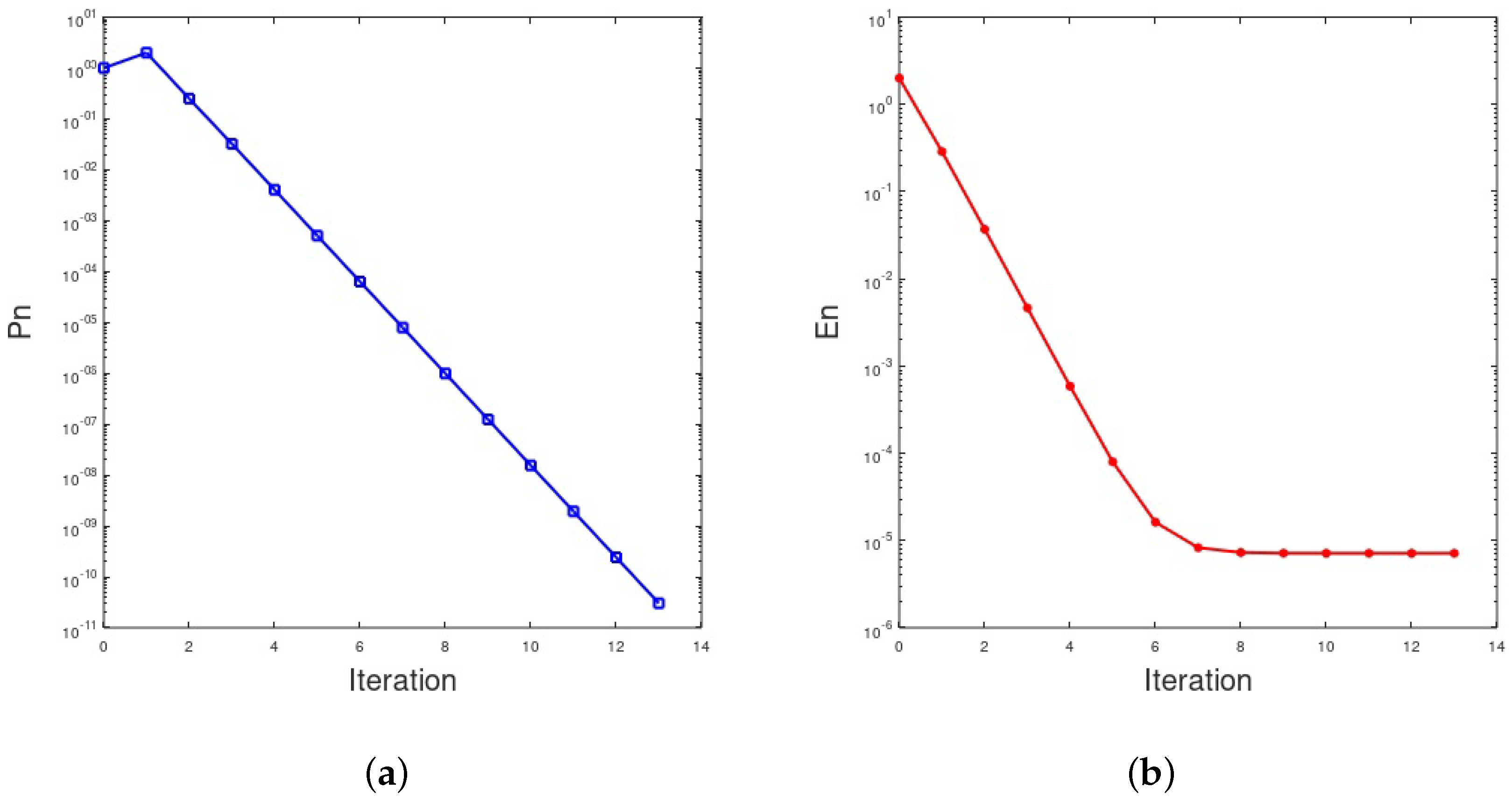
Let us choose $x_0\left(s\right)=5$ and $x_{-1}\left(s\right)=6$. Both methods give approximate solution of the integral equation under 13 iterations for $\epsilon ={10}^{-10}$. To solve a linear integral equation at each iteration was applied Nystrom method. We use a trapezoidal quadrature formula with 101 nodes. On the graphs $P_n$ denotes $\parallel x_n-x_{n-1}\parallel$ and $E_n$ denotes $\parallel x_n-x_{*}\parallel$ (see Figure 1). We can see that $E_n=O\left(h^2\right)$, where $h=0.01$. This corresponds to the error estimation of the trapezoidal quadrature formula.

7. Conclusions

The investigations conducted showed the effectiveness of applying the Kantorovich majorant principle for determining the convergence and the order of convergence of iterative difference methods. The convergence of the Secant method (2) with the order ${\displaystyle \frac{1+\sqrt{5}}{2}}$ and the quadratic convergence order of the Kurchatov’s method (3) are established. According to this technique, nonlinear majorants for a nonlinear operator are constructed, taking into account the conditions imposed on it. By using our idea of restricted convergence regions, we find tighter Lipschitz constants leading to a finer local convergence analysis of these methods than in [1]. Our new technique can be used to extend the applicability of other methods along the same lines. More details on the extensions were given in Remark 1.

References

- Shakhno, S.M. Nonlinear majorants for investigation of methods of linear interpolation for the solution of nonlinear equations. In Proceedings of the ECCOMAS 2004—European Congress on Computational Methods in Applied Sciences and Engineering, Jyväskylä, Finland, 24–28 July 2004; Available online: http://www.mit.jyu.fi/eccomas2004/proceedings/pdf/424.pdf (accessed on 26 May 2020).
- Amat, S. On the local convergence of secant-type methods. Int. J. Comput. Math. 2004, 81, 1153–1161. [Google Scholar] [CrossRef]
- Hernandez, M.A.; Rubio, M.J. The Secant method for nondifferentiable operators. Appl. Math. Lett. 2002, 15, 395–399. [Google Scholar] [CrossRef] [Green Version]
- Shakhno, S.; Gnatyshyn, O. Iterative-Difference Methods for Solving Nonlinear Least-Squares Problem. In Progress in Industrial Mathematics at ECMI 98; Arkeryd, L., Bergh, J., Brenner, P., Pettersson, R., Eds.; Verlag B. G. Teubner GMBH: Stuttgart, Germany, 1999; pp. 287–294. [Google Scholar]
- Ul’m, S. Algorithms of the generalized Steffensen method. Izv. Akad. Nauk ESSR Ser. Fiz.-Mat. 1965, 14, 433–443. (In Russian) [Google Scholar]
- Ul’m, S. On generalized divided differences I, II. Izv. Akad. Nauk ESSR Ser. Fiz.-Mat. 1967, 16, 13–26. (In Russian) [Google Scholar]
- Kantorovich, L.V.; Akilov, G.P. Functional Analysis; Pergamon Press: Oxford, UK, 1982. [Google Scholar]
- Potra, F.A. On an iterative algorithm of order 1.839... for solving nonlinear operator equations. Numer. Funct. Anal. Optim. 1985, 7, 75–106. [Google Scholar] [CrossRef]
- Ul’m, S. Iteration methods with divided differences of the second order. Doklady Akademii Nauk SSSR 1964, 158, 55–58. [Google Scholar]
- Schwetlick, H. Numerische Lösung Nichtlinearer Gleichungen; VEB Deutscher Verlag der Wissenschaften: Berlin, Germany, 1979. [Google Scholar]
- Argyros, I.K. A Kantorovich-type analysis for a fast iterative method for solving nonlinear equations. J. Math. Anal. Appl. 2007, 332, 97–108. [Google Scholar] [CrossRef] [Green Version]
- Argyros, I.K.; George, S. On a two-step Kurchatov-type method in Banach space. Mediterr. J. Math. 2019, 16. [Google Scholar] [CrossRef]
- Argyros, I.K.; Magreñán, A.A. Iterative Methods and Their Dynamics with Applications: A Contemporary Study; CRC Press: Boca Raton, FL, USA, 2017. [Google Scholar]
- Kurchatov, V.A. On a method of linear interpolation for the solution of functional equations. Dokl. Akad. Nauk SSSR 1971, 198, 524–526. [Google Scholar]
- Shakhno, S.M. Kurchatov method of linear interpolation under generalized Lipschitz conditions for divided differences of first and second order. Visnyk Lviv. Univ. Ser. Mech. Math. 2012, 77, 235–242. (In Ukrainian) [Google Scholar]
- Shakhno, S.M. On the difference method with quadratic convergence for solving nonlinear operator equations. Matematychni Studii 2006, 26, 105–110. (In Ukrainian) [Google Scholar]
Figure 1.
Values of (a) and (b)
at each iteration.