Multi-Scale Evaluation of the TSEB Model over a Complex Agricultural Landscape in Morocco

 ,
,  ,
,  ,
,  ,
, 

Abstract
:1. Introduction
2. Materials and Methods
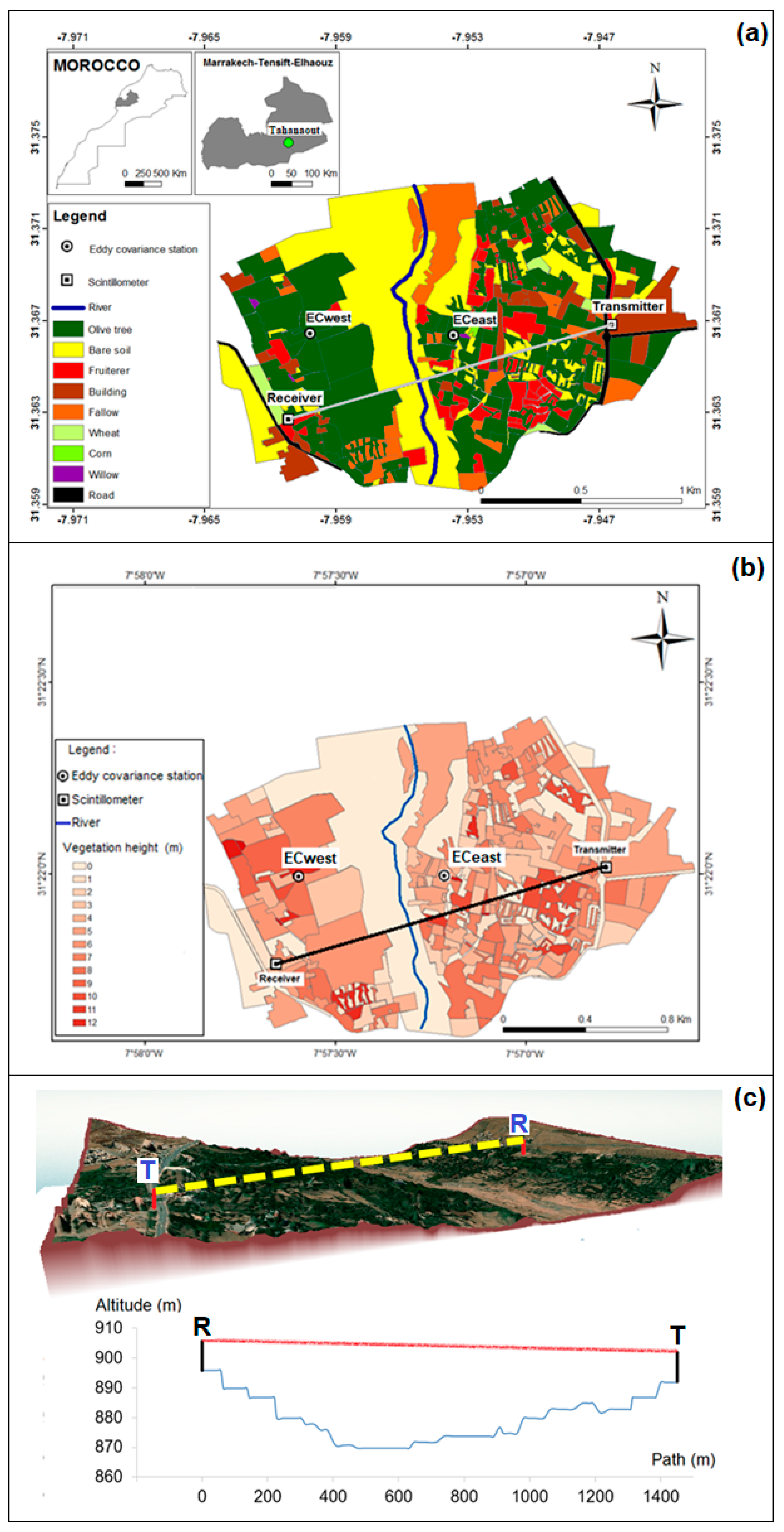
2.1. Site and Experimental Data
2.2. Scintillometry Theoretical Background
2.2.1. Determining the Sensible and Latent Heat Flux from LAS
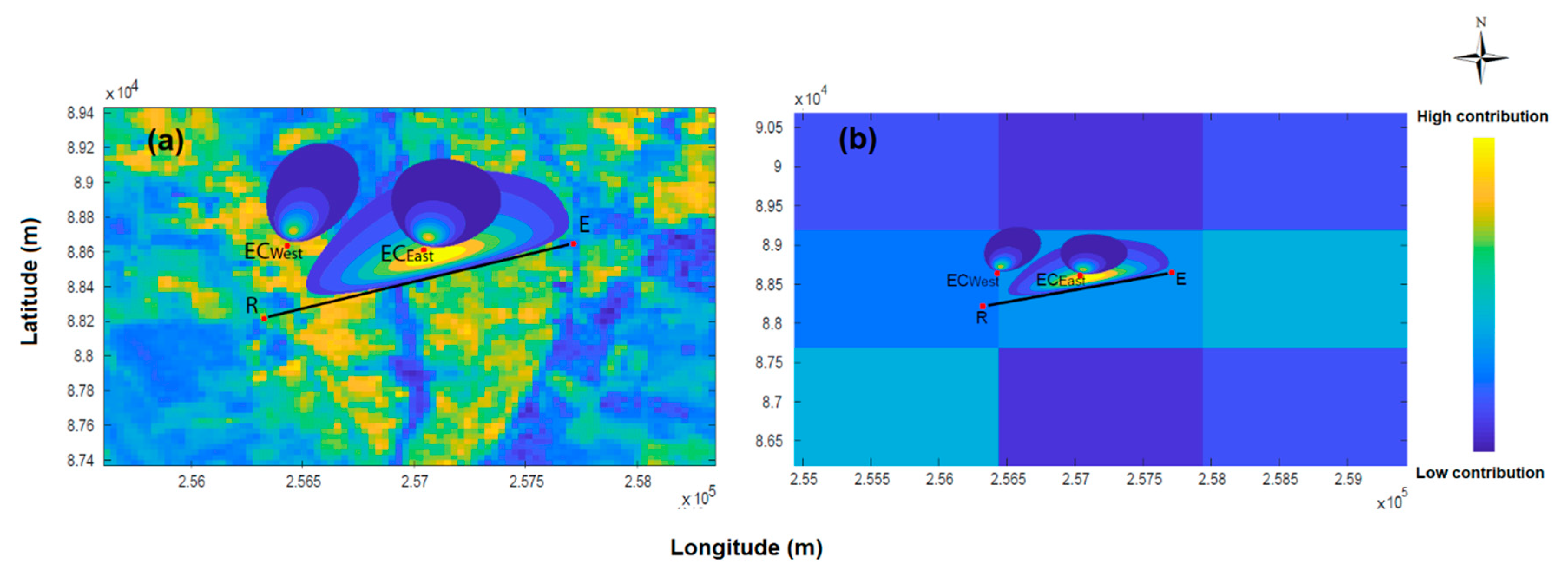
2.2.2. Scintillometer Footprint
2.3. The Two-Source Energy Balance Model
2.4. Satellite Products and Data
2.4.1. MODIS Products
2.4.2. Landsat Products
3. Results and Discussion
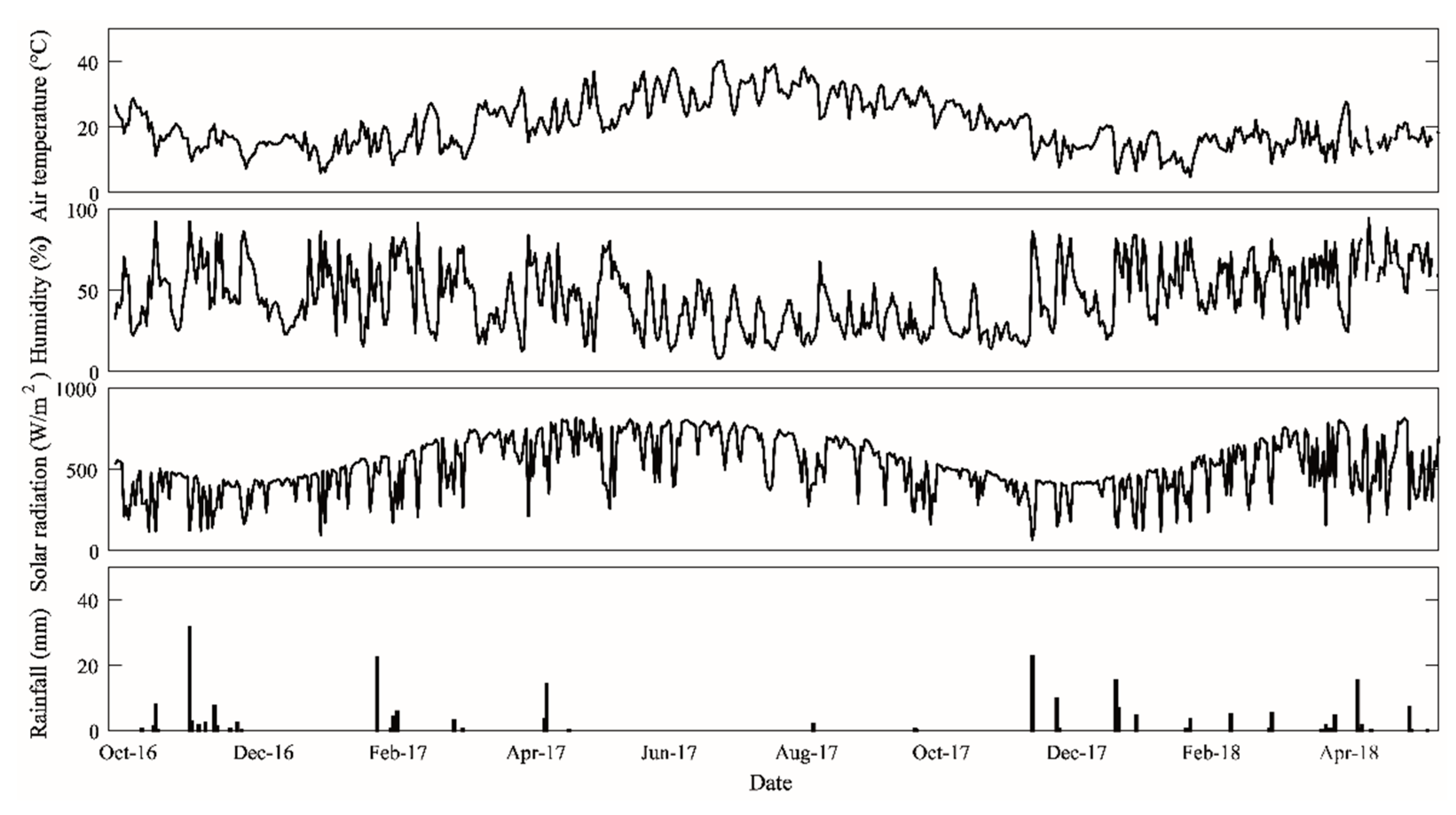
3.1. Experimental Data Analysis
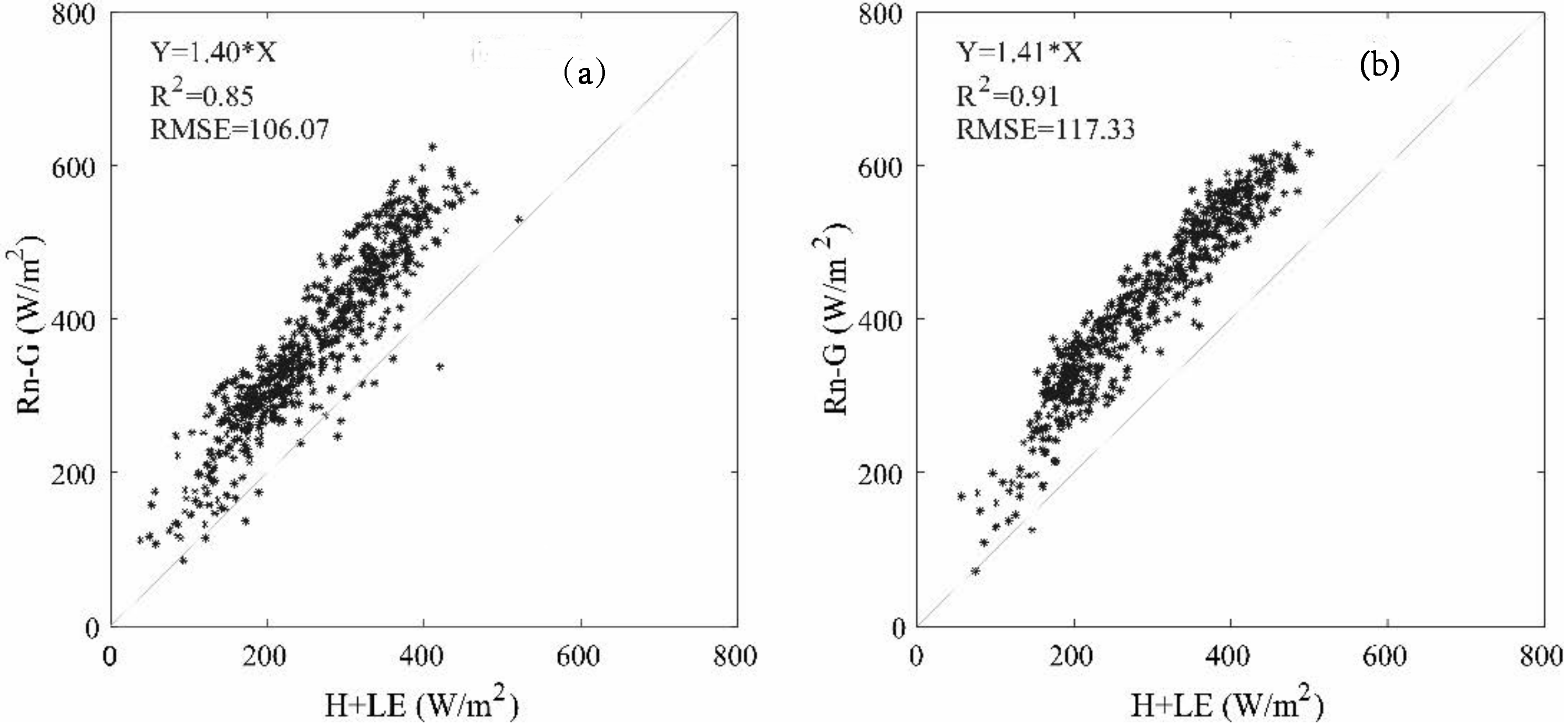
3.1.1. Energy Balance Closure
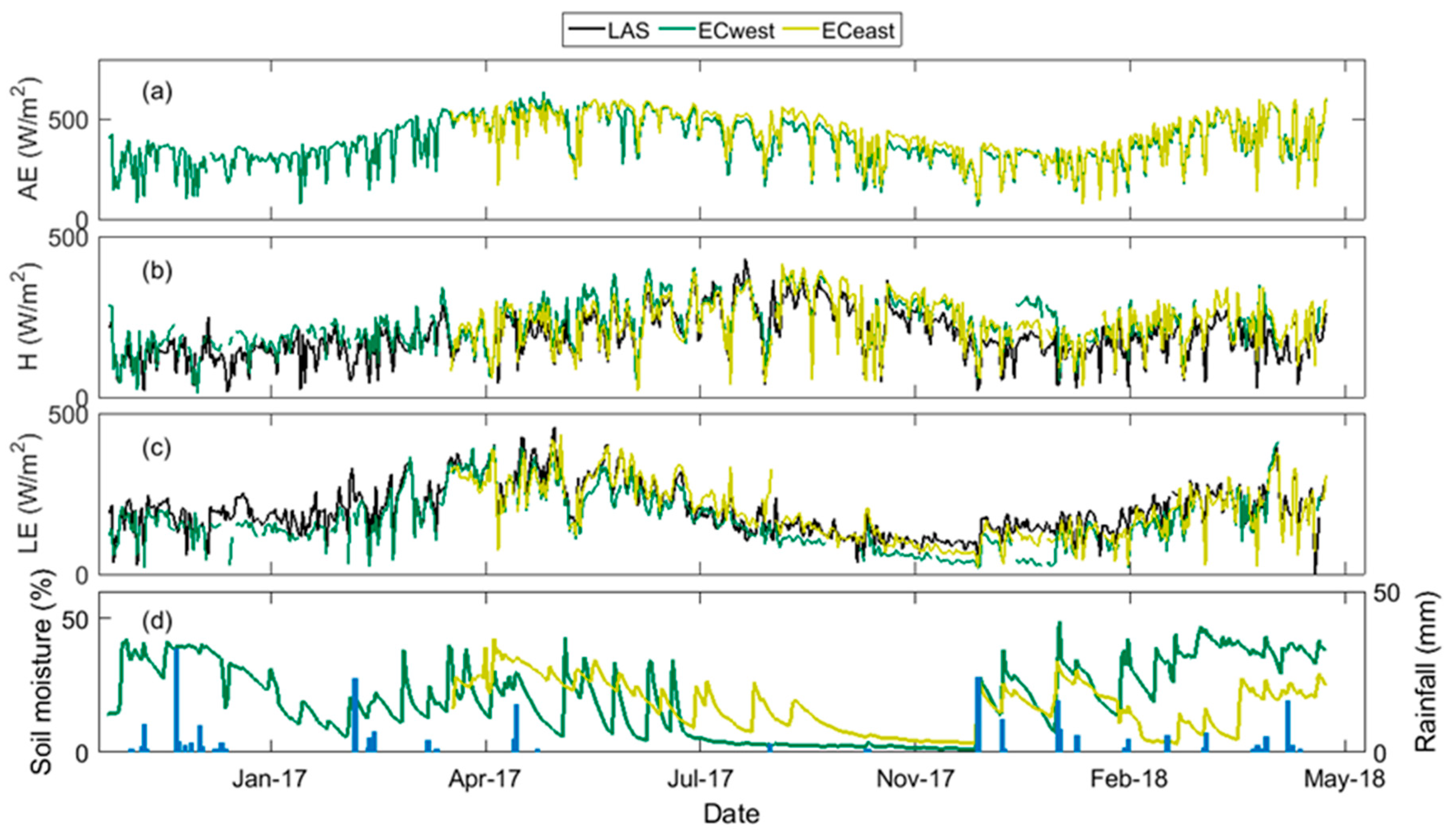
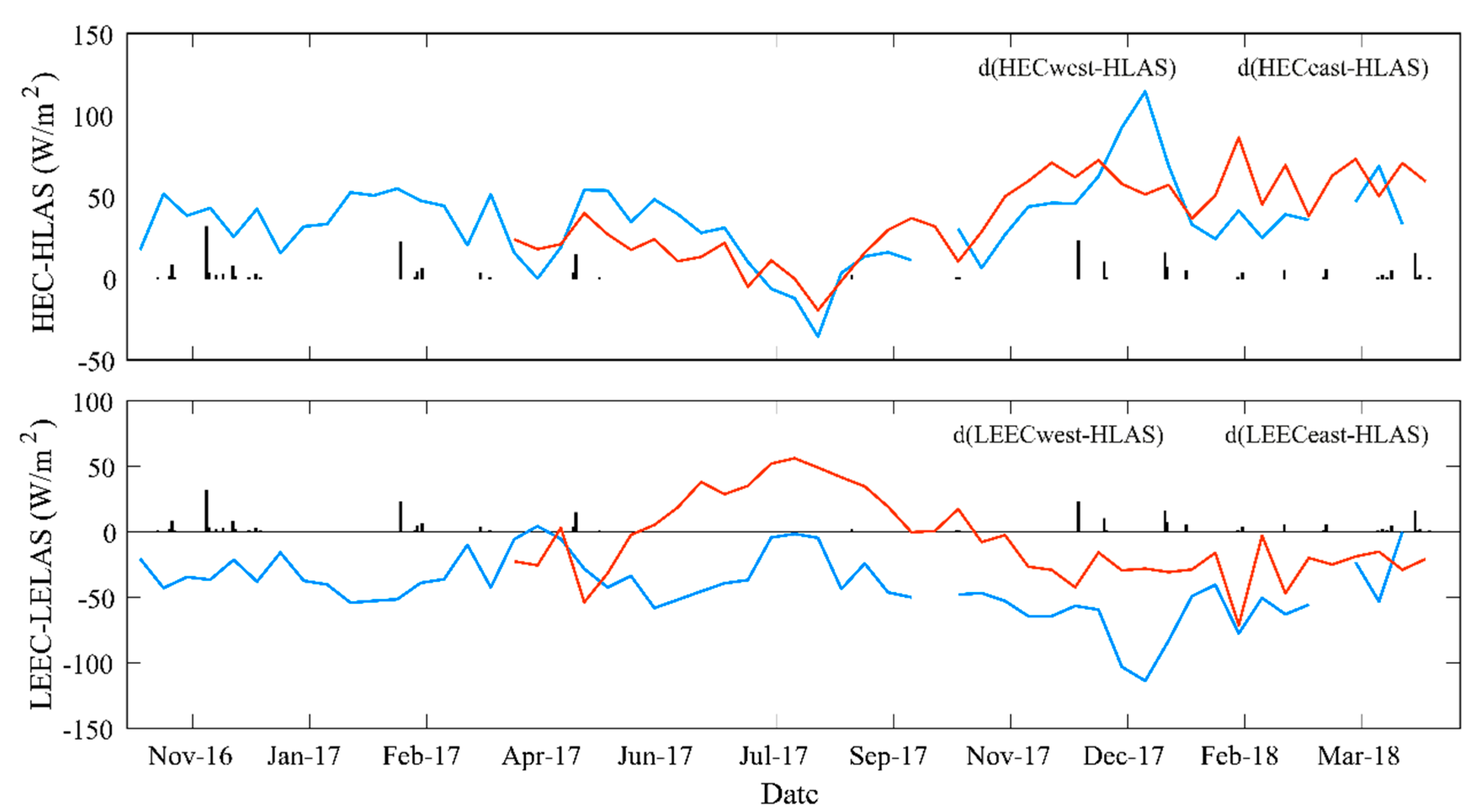
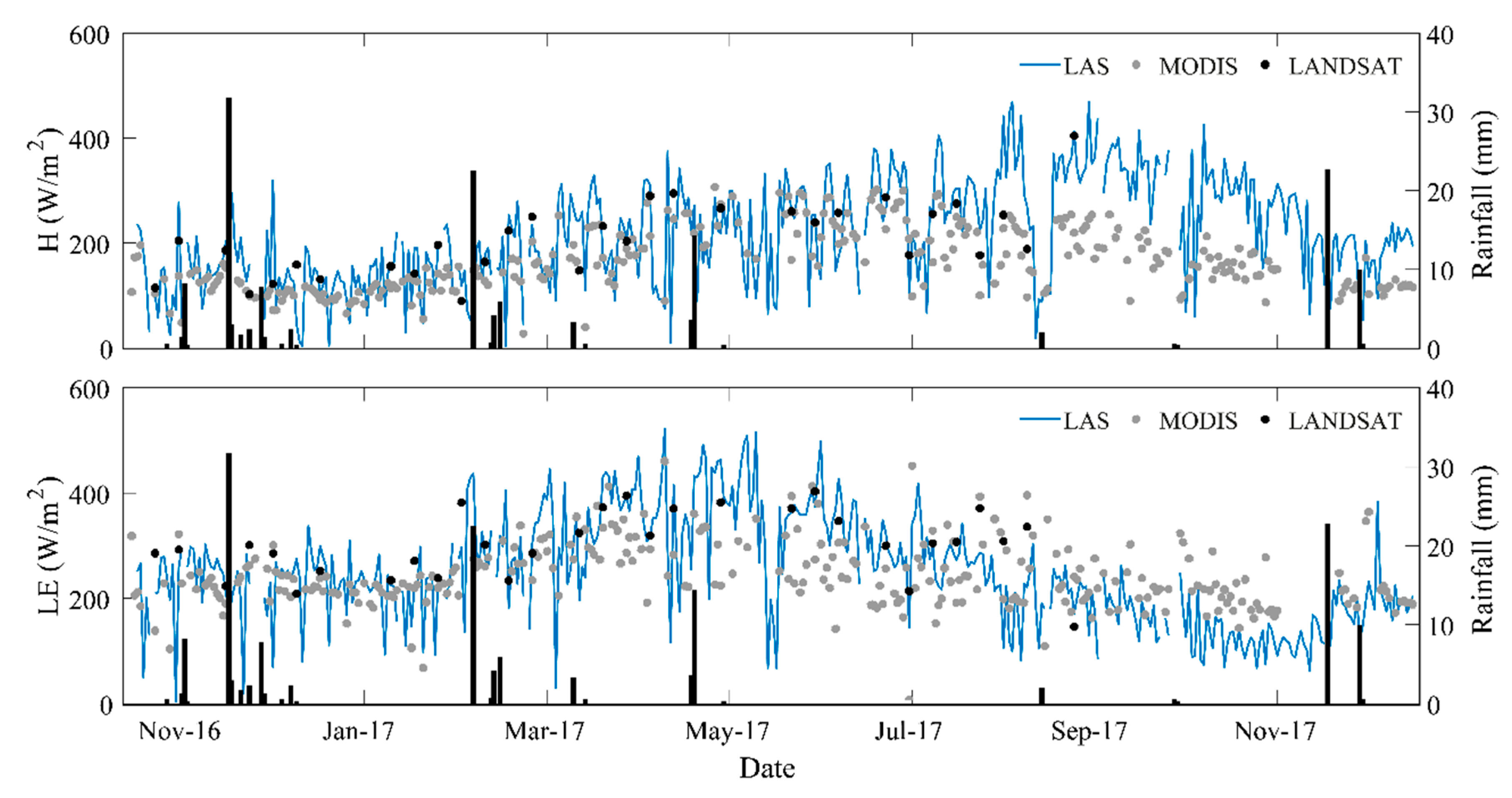
3.1.2. Seasonal Course of Convective Fluxes
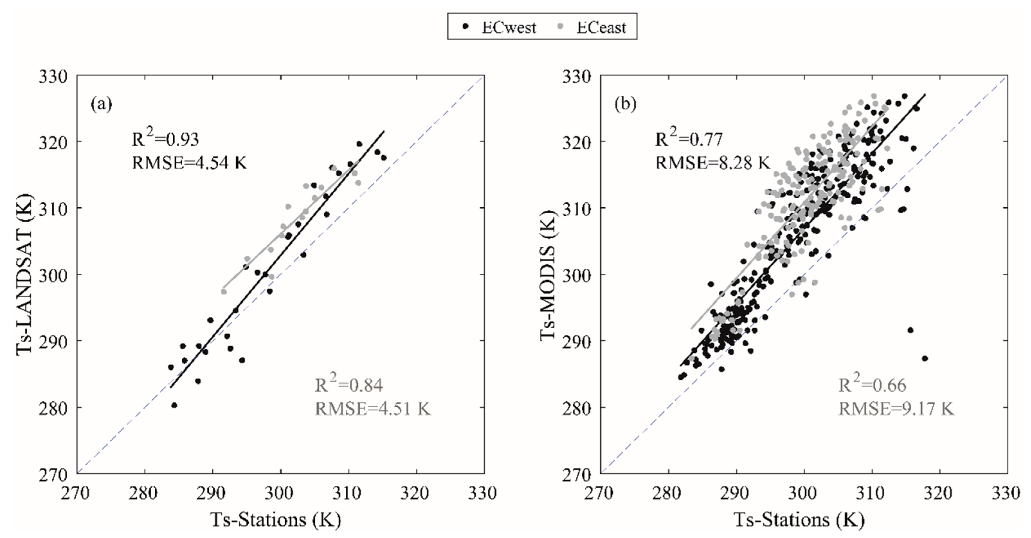
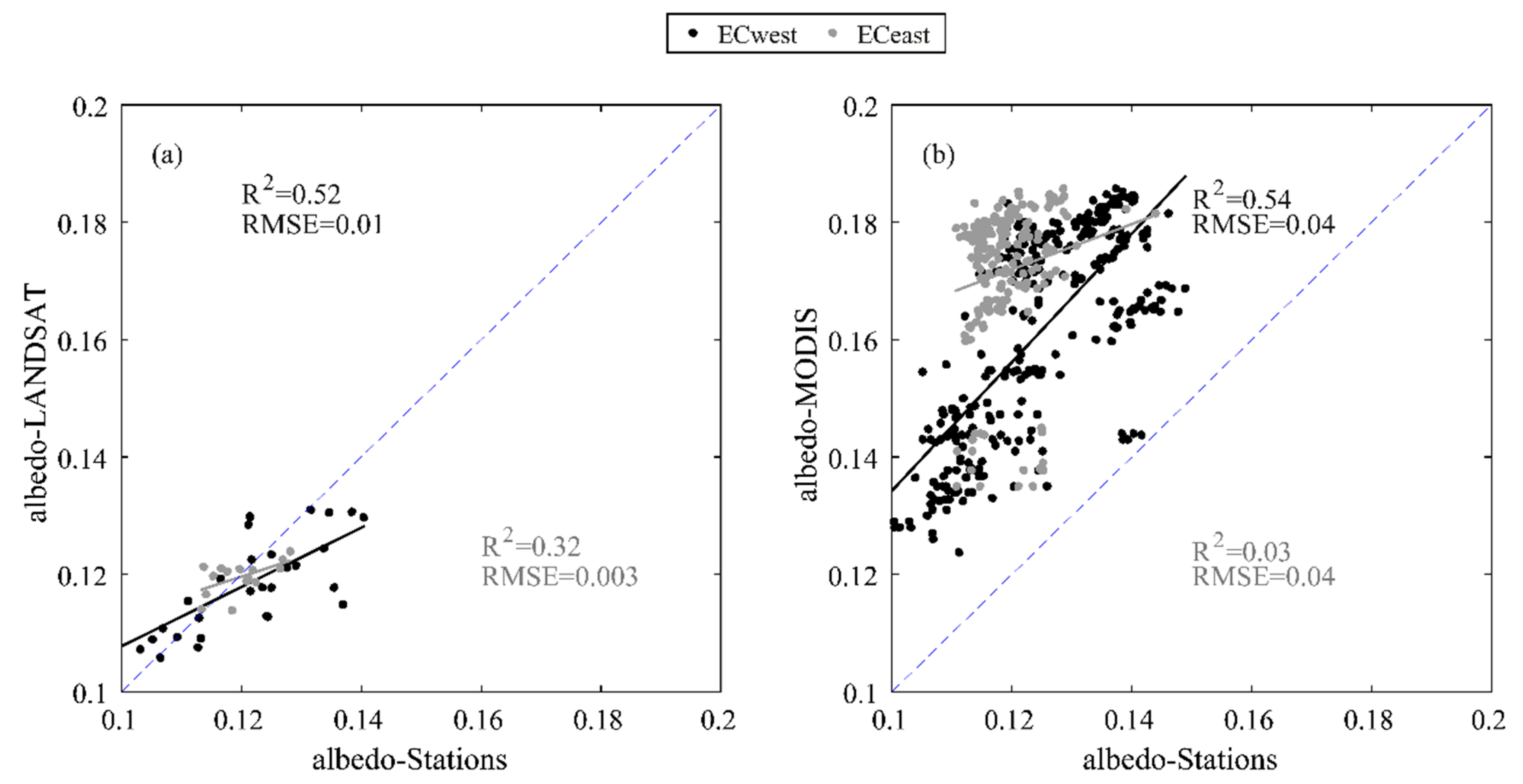
3.2. Evaluation of Satellites Products
3.3. TSEB Results
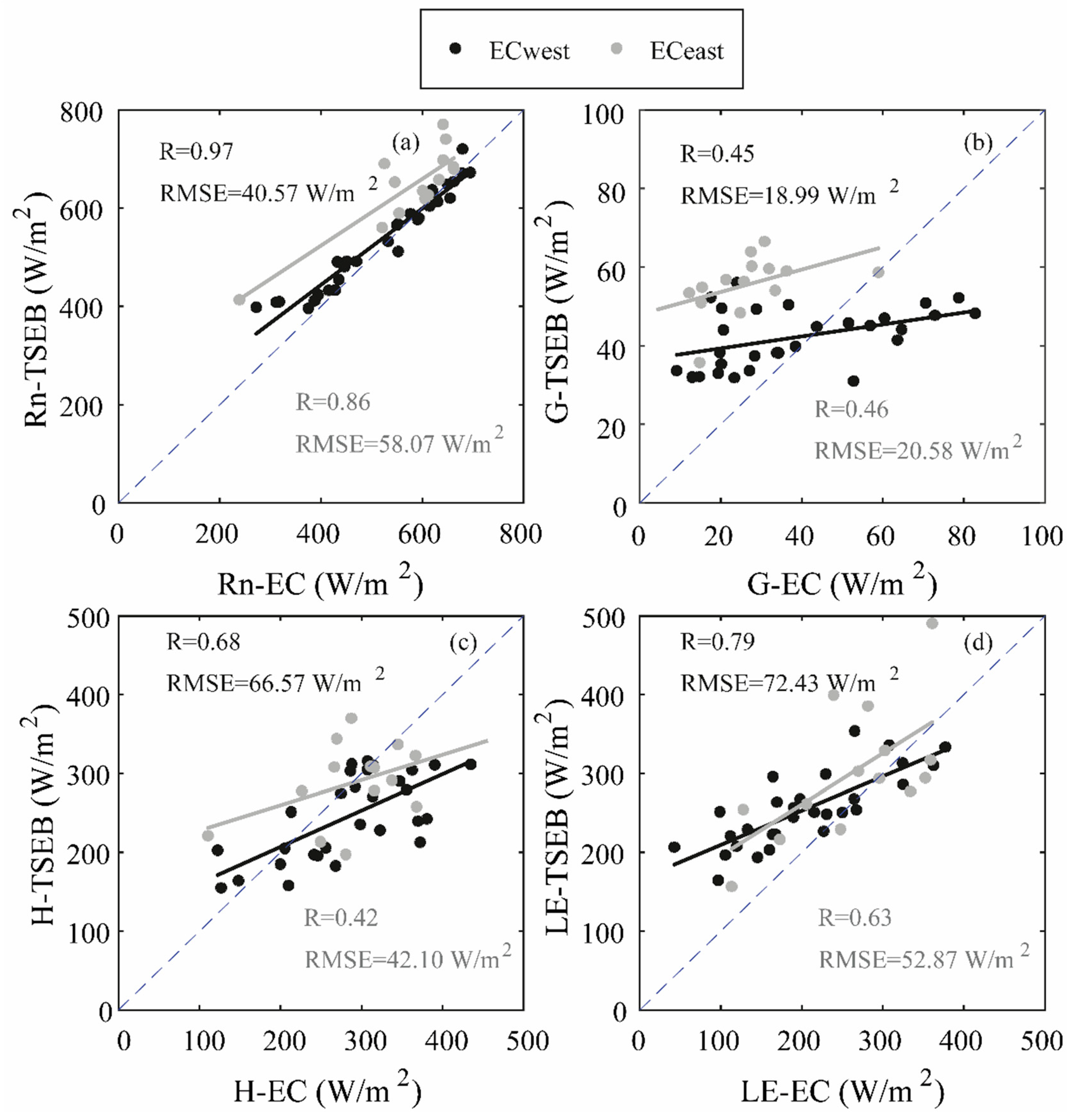
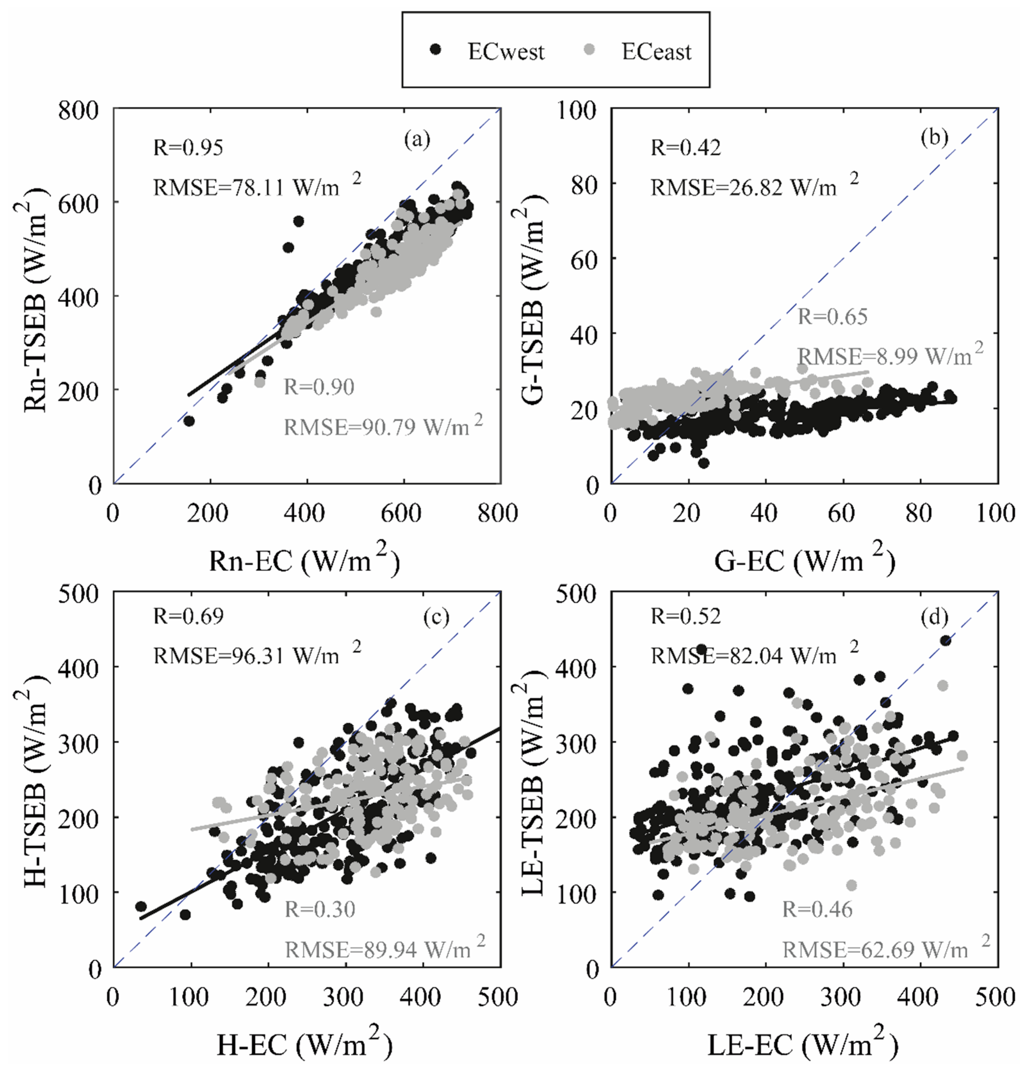
3.3.1. Field Scale
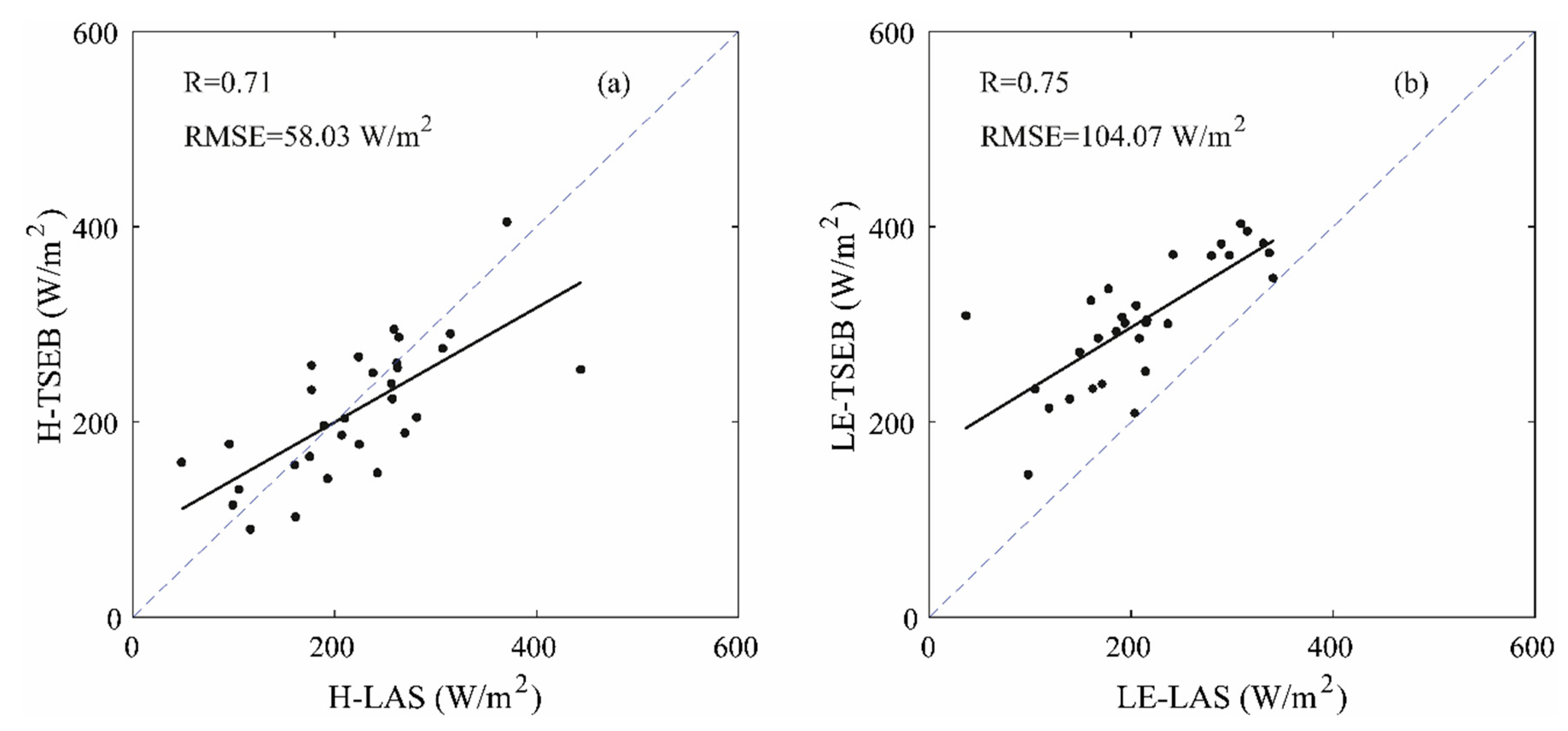
3.3.2. Multi-Field Scale
4. Conclusions
Author Contributions
Funding
Acknowledgments
Conflicts of Interest
References
- Giorgi, F. Climate change hot-spots. Geophys. Res. Lett. 2006, 33. [Google Scholar] [CrossRef]
- Glenn, E.P.; Huete, A.R.; Nagler, P.L.; Hirschboeck, K.K.; Brown, P. Integrating remote sensing and ground methods to estimate evapotranspiration. CRC Crit. Rev. Plant Sci. 2007, 26, 139–168. [Google Scholar] [CrossRef]
- Jasechko, S.; Sharp, Z.D.; Gibson, J.J.; Birks, S.J.; Yi, Y.; Fawcett, P.J. Terrestrial water fluxes dominated by transpiration. Nature 2013, 496, 347–350. [Google Scholar] [CrossRef] [PubMed]
- Ezzahar, J.; Chehbouni, A.; Hoedjes, J.C.B.; Er-Raki, S.; Chehbouni, A.; Boulet, G.; Bonnefond, J.M.; De Bruin, H.A.R. The use of the scintillation technique for monitoring seasonal water consumption of olive orchards in a semi-arid region. Agric. Water Manag. 2007, 89, 173–184. [Google Scholar] [CrossRef] [Green Version]
- Ezzahar, J.; Chehbouni, A.; Hoedjes, J.C.B.; Chehbouni, A. On the application of scintillometry over heterogeneous grids. J. Hydrol. 2007, 334, 493–501. [Google Scholar] [CrossRef] [Green Version]
- Ezzahar, J.; Chehbouni, A.; Er-Raki, S.; Hanich, L. Combining a large aperture scintillometer and estimates of available energy to derive evapotranspiration over several agricultural fields in a semi-arid region. Plant Biosyst. 2009, 143, 209–221. [Google Scholar] [CrossRef] [Green Version]
- Ezzahar, J.; Chehbouni, A.; Hoedjes, J.; Ramier, D.; Boulain, N.; Boubkraoui, S.; Cappelaere, B.; Descroix, L.; Mougenot, B.; Timouk, F. Combining scintillometer measurements and an aggregation scheme to estimate area-averaged latent heat flux during the AMMA experiment. J. Hydrol. 2009, 375, 217–226. [Google Scholar] [CrossRef] [Green Version]
- Er-Raki, S.; Chehbouni, A.; Duchemin, B. Combining satellite remote sensing data with the FAO-56 dual approach for water use mapping in irrigated wheat fields of a semi-arid region. Remote Sens. 2010, 2, 375–387. [Google Scholar] [CrossRef] [Green Version]
- Diarra, A.; Jarlan, L.; Er-Raki, S.; Le Page, M.; Aouade, G.; Tavernier, A.; Boulet, G.; Ezzahar, J.; Merlin, O.; Khabba, S. Performance of the two-source energy budget (TSEB) model for the monitoring of evapotranspiration over irrigated annual crops in North Africa. Agric. Water Manag. 2017, 193, 71–88. [Google Scholar] [CrossRef]
- Hssaine, B.A.; Merlin, O.; Rafi, Z.; Ezzahar, J.; Jarlan, L.; Khabba, S.; Er-Raki, S. Calibrating an evapotranspiration model using radiometric surface temperature, vegetation cover fraction and near-surface soil moisture data. Agric. For. Meteorol. 2018, 256–257, 104–115. [Google Scholar] [CrossRef] [Green Version]
- Rafi, Z.; Merlin, O.; Le Dantec, V.; Khabba, S.; Mordelet, P.; Er-Raki, S.; Amazirh, A.; Olivera-Guerra, L.; Ait Hssaine, B.; Simonneaux, V.; et al. Partitioning evapotranspiration of a drip-irrigated wheat crop: Inter-comparing eddy covariance-, sap flow-, lysimeter- and FAO-based methods. Agric. For. Meteorol. 2019, 265, 310–326. [Google Scholar] [CrossRef]
- Lee, X.; Finnigan, J.; Paw U, K.T. Handbook of Micrometeorology: A Guide for Surface Flux Measurement and Analysis; Springer: Berlin, Germany, 2005; Volume 29, pp. 33–66. [Google Scholar] [CrossRef]
- Foken, T. The energy balance closure problem: An overview. Ecol. Appl. 2008, 18, 1351–1367. [Google Scholar] [CrossRef]
- Zeweldi, D.A.; Gebremichael, M.; Wang, J.; Sammis, T.; Kleissl, J.; Miller, D. Intercomparison of sensible heat flux from large aperture scintillometer and eddy covariance methods: Field experiment over a homogeneous semi-arid region. Bound.-Layer Meteorol. 2010, 135, 151–159. [Google Scholar] [CrossRef] [Green Version]
- Vesala, T.; Eugster, W.; Ojala, A. Eddy Covariance Measurements over Lakes. In Eddy Covariance: A Practical Guide to Measurement and Data Analysis; Springer: Berlin, Germany, 2012; pp. 365–376. [Google Scholar] [CrossRef]
- Odhiambo, G.O.; Savage, M.J. Sensible heat flux by surface layer scintillometry and eddy covariance over a mixed grassland community as affected by Bowen ratio and MOST formulations for unstable conditions. J. Hydrometeorol. 2009, 10, 479–492. [Google Scholar] [CrossRef]
- Jacobs, C.; Elbers, J.; Brolsma, R.; Hartogensis, O.; Moors, E.; Rodríguez-Carretero Márquez, M.T.; van Hove, B. Assessment of evaporative water loss from Dutch cities. Build. Environ. 2015, 83, 27–38. [Google Scholar] [CrossRef]
- Crawford, B.; Grimmond, C.S.B.; Ward, H.C.; Morrison, W.; Kotthaus, S. Spatial and temporal patterns of surface–atmosphere energy exchange in a dense urban environment using scintillometry. Q. J. R. Meteorol. Soc. 2017, 143, 817–833. [Google Scholar] [CrossRef] [Green Version]
- Rotach, M.W.; Stiperski, I.; Fuhrer, O.; Goger, B.; Gohm, A.; Obleitner, F.; Rau, G.; Sfyri, E.; Vergrgeiner, J. Investigating exchange processes over complex topography: The Innsbruck box (i-Box). Bull. Am. Meteorol. Soc. 2017, 98, 787–805. [Google Scholar] [CrossRef]
- Duchemin, B.; Hagolle, O.; Mougenot, B.; Benhadj, I.; Hadria, R.; Simonneaux, V.; Ezzahar, J.; Hoedjes, J.; Khabba, S.; Kharrou, M.H.; et al. Agrometerological study of semi-ard areas: An experiment for analysing the potential of time series of FORMOSAT-2 images (Tensift-Marrakech plain). Int. J. Remote Sens. 2008, 29, 5291–5300. [Google Scholar] [CrossRef] [Green Version]
- Hssaine, B.A.; Ezzahar, J.; Jarlan, L.; Merlin, O.; Khabba, S.; Brut, A.; Er-Raki, S.; Elfarkh, J.; Cappelaere, B.; Chehbouni, G. Combining a two source energy balance model driven by MODIS and MSG-SEVIRI products with an aggregation approach to estimate turbulent fluxes over sparse and heterogeneous vegetation in Sahel region (Niger). Remote Sens. 2018, 10, 974. [Google Scholar] [CrossRef] [Green Version]
- Hoedjes, J.C.B.; Chehbouni, A.; Ezzahar, J.; Escadafal, R.; De Bruin, H.A.R. Comparison of Large Aperture Scintillometer and Eddy Covariance Measurements: Can Thermal Infrared Data Be Used to Capture Footprint-Induced Differences? J. Hydrometeorol. 2007, 8, 144–159. [Google Scholar] [CrossRef] [Green Version]
- Ezzahar, J.; Chehbouni, A. The use of scintillometry for validating aggregation schemes over heterogeneous grids. Agric. For. Meteorol. 2009, 149, 2098–2109. [Google Scholar] [CrossRef] [Green Version]
- Saadi, S.; Boulet, G.; Bahir, M.; Brut, A.; Delogu, É.; Fanise, P.; Mougenot, B.; Simonneaux, V.; Chabaane, Z.L. Assessment of actual evapotranspiration over a semiarid heterogeneous land surface by means of coupled low-resolution remote sensing data with an energy balance model: Comparison to extra-large aperture scintillometer measurements. Hydrol. Earth Syst. Sci. 2018, 22, 2187–2209. [Google Scholar] [CrossRef] [Green Version]
- Kustas, W.; Anderson, M. Advances in thermal infrared remote sensing for land surface modeling. Agric. For. Meteorol. 2009, 149, 2071–2081. [Google Scholar] [CrossRef]
- Ma, Y.; Zhu, Z.; Zhong, L.; Wang, B.; Han, C.; Wang, Z.; Wang, Y.; Lu, L.; Amatya, P.M.; Ma, W.; et al. Combining MODIS, AVHRR and in situ data for evapotranspiration estimation over heterogeneous landscape of the Tibetan Plateau. Atmos. Chem. Phys. 2014, 14, 1507–1515. [Google Scholar] [CrossRef] [Green Version]
- Song, L.; Liu, S.; Zhang, X.; Zhou, J.; Li, M. Estimating and validating soil evaporation and crop transpiration during the HiWATER-MUSOEXE. IEEE Geosci. Remote Sens. Lett. 2015, 12, 334–338. [Google Scholar] [CrossRef] [Green Version]
- Castelli, M.; Anderson, M.C.; Yang, Y.; Wohlfahrt, G.; Bertoldi, G.; Niedrist, G.; Hammerle, A.; Zhao, P.; Zebisch, M.; Notarnicola, C. Two-source energy balance modeling of evapotranspiration in Alpine grasslands. Remote Sens. Environ. 2018, 209, 327–342. [Google Scholar] [CrossRef]
- Su, Z. The Surface Energy Balance System (SEBS) for estimation of turbulent heat fluxes. Hydrol. Earth Syst. Sci. 2002, 6, 85–100. [Google Scholar] [CrossRef]
- Allen, R.G.; Tasumi, M.; Morse, A.; Trezza, R.; Wright, J.L.; Bastiaanssen, W.; Kramber, W.; Lorite, I.J.; Robison, C.W. Journal of Irrigation and Drainage Engineering Satellite-Based Energy Balance for Mapping Evapotranspiration with Internalized Calibration (METRIC)— Applications. J. Irrig. Drain. Eng. 2007, 133, 395–406. [Google Scholar] [CrossRef]
- Bastiaanssen, W.G.M.; Pelgrum, H.; Wang, J.; Ma, Y.; Moreno, J.F.; Roerink, G.J.; Van Der Wal, T. A remote sensing surface energy balance algorithm for land (SEBAL): 2. Validation. J. Hydrol. 1998, 212–213, 213–229. [Google Scholar] [CrossRef]
- Norman, J.M.; Kustas, W.P.; Humes, K.S. Source approach for estimating soil and vegetation energy fluxes in observations of directional radiometric surface temperature. Agric. For. Meteorol. 1995, 77, 263–293. [Google Scholar] [CrossRef]
- Boulet, G.; Mougenot, B.; Lhomme, J.P.; Fanise, P.; Lili-Chabaane, Z.; Olioso, A.; Bahir, M.; Rivalland, V.; Jarlan, L.; Merlin, O.; et al. The SPARSE model for the prediction of water stress and evapotranspiration components from thermal infra-red data and its evaluation over irrigated and rainfed wheat. Hydrol. Earth Syst. Sci. 2015, 19, 4653–4672. [Google Scholar] [CrossRef] [Green Version]
- Anderson, M.; Kustas, W. Thermal Remote Sensing of Drought and Evapotranspiration.pdf. Eos Trans. Am. Geophys. Union 2008, 89, 233–240. [Google Scholar] [CrossRef]
- Choi, M.; Kustas, W.P.; Anderson, M.C.; Allen, R.G.; Li, F.; Kjaersgaard, J.H. An intercomparison of three remote sensing-based surface energy balance algorithms over a corn and soybean production region (Iowa, U.S.) during SMACEX. Agric. For. Meteorol. 2009, 149, 2082–2097. [Google Scholar] [CrossRef]
- French, A.N.; Jacob, F.; Anderson, M.C.; Kustas, W.P.; Timmermans, W.; Gieske, A.; Su, Z.; Su, H.; McCabe, M.F.; Li, F.; et al. Surface energy fluxes with the Advanced Spaceborne Thermal Emission and Reflection radiometer (ASTER) at the Iowa 2002 SMACEX site (USA). Remote Sens. Environ. 2005, 99, 55–65. [Google Scholar] [CrossRef]
- Gonzalez-Dugo, M.P.; Neale, C.M.U.; Mateos, L.; Kustas, W.P.; Prueger, J.H.; Anderson, M.C.; Li, F. A comparison of operational remote sensing-based models for estimating crop evapotranspiration. Agric. For. Meteorol. 2009, 149, 1843–1853. [Google Scholar] [CrossRef]
- Kustas, W.P.; Norman, J.M. A two-source energy balance approach using directional radiometric temperature observations for sparse canopy covered surfaces. Agron. J. 2000, 92, 847–854. [Google Scholar] [CrossRef]
- Timmermans, W.J.; Kustas, W.P.; Anderson, M.C.; French, A.N. An intercomparison of the Surface Energy Balance Algorithm for Land (SEBAL) and the Two-Source Energy Balance (TSEB) modeling schemes. Remote Sens. Environ. 2007, 108, 369–384. [Google Scholar] [CrossRef]
- Tang, R.; Li, Z.L.; Jia, Y.; Li, C.; Sun, X.; Kustas, W.P.; Anderson, M.C. An intercomparison of three remote sensing-based energy balance models using Large Aperture Scintillometer measurements over a wheat-corn production region. Remote Sens. Environ. 2011, 115, 3187–3202. [Google Scholar] [CrossRef]
- Tang, R.; Li, Z.L. An End-Member-Based Two-Source Approach for Estimating Land Surface Evapotranspiration from Remote Sensing Data. IEEE Trans. Geosci. Remote Sens. 2017, 55, 5818–5832. [Google Scholar] [CrossRef]
- Kustas, W.P.; Norman, J.M. Evaluation of soil and vegetation heat flux predictions using a simple two-source model with radiometric temperatures for partial canopy cover. Agric. For. Meteorol. 1999, 94, 13–29. [Google Scholar] [CrossRef]
- Anderson, M.C.; Norman, J.M.; Diak, G.R.; Kustas, W.P.; Mecikalski, J.R. A two-source time-integrated model for estimating surface fluxes using thermal infrared remote sensing. Remote Sens. Environ. 1997, 60, 195–216. [Google Scholar] [CrossRef]
- Lagouarde, J.P.; Bhattacharya, B.K.; Crébassol, P.; Gamet, P.; Babu, S.S.; Boulet, G.; Briottet, X.; Buddhiraju, K.M.; Cherchali, S.; Dadou, I.; et al. The Indian-French Trishna mission: Earth observation in the thermal infrared with high spatio-temporal resolution. In Proceedings of the International Geoscience and Remote Sensing Symposium (IGARSS), Valencia, Spain, 22–27 July 2018; pp. 4078–4081. [Google Scholar]
- Hartogensis, O.K.; Watts, C.J.; Rodriguez, J.-C.; De Bruin, H.A.R. Derivation of an Effective Height for Scintillometers: La Poza Experiment in Northwest Mexico. J. Hydrometeorol. 2003, 4, 915–928. [Google Scholar] [CrossRef]
- Wesely, M.L. Combined effect of temperature and humidity fluctuations on refractive index. J. Appl. Meteorol. 1976, 15, 43–49. [Google Scholar] [CrossRef]
- Solignac, P.A.; Brut, A.; Selves, J.-L.; Béteille, J.-P.; Gastellu-Etchegorry, J.-P.; Keravec, P.; Béziat, P.; Ceschia, E. Uncertainty analysis of computational methods for deriving sensible heat flux values from scintillometer measurements. Atmos. Meas. Tech. 2009, 2, 741–753. [Google Scholar] [CrossRef] [Green Version]
- De Bruin, H.A.R.; Kohsiek, W.; Van Den Hurk, B.J.J.M. A verification of some methods to determine the fluxes of momentum, sensible heat, and water vapour using standard deviation and structure parameter of scalar meteorological quantities. Bound.-Layer Meteorol. 1993, 53, 231–257. [Google Scholar] [CrossRef]
- Panofsky, H.A.; Jensen, N.O.; Jackson, P.S. Introduction to wind characteristics: Flow over hills and ridges. In Wind Engineering 1983; Elsevier: Amsterdam, The Netherlands, 1984. [Google Scholar] [CrossRef]
- Brutsaert, W. Evaporation into the atmosphere. Theory, history, and applications; Springer: Dordrecht, The Netherlands, 1982; pp. 1223–1224. [Google Scholar] [CrossRef]
- Horst, T.W.; Weil, J.C. Footprint estimation for scalar flux measurements in the atmospheric surface layer. Bound.-Layer Meteorol. 1992, 59, 279–296. [Google Scholar] [CrossRef]
- Horst, T.W.; Weil, J.C. How far is far enough? The fetch requirements for micrometeorological measurement of surface fluxes. J. Atmos. Ocean. Technol. 1994, 11, 1018–1025. [Google Scholar] [CrossRef] [Green Version]
- Schuepp, P.H.; Leclerc, M.Y.; MacPherson, J.I.; Desjardins, R.L. Footprint prediction of scalar fluxes from analytical solutions of the diffusion equation. Bound.-Layer Meteorol. 1990, 50, 355–373. [Google Scholar] [CrossRef]
- Rannik, U.; Aubinet, M.; Kurbanmuradov, O.; Sabelfeld, K.K.; Markkanen, T.; Vesala, T. Footprint analysis for measurements over a heterogeneous forest. Bound.-Layer Meteorol. 2000, 97, 137–166. [Google Scholar] [CrossRef]
- Meijninger, W.M.L. Surface Fluxes over Natural Landscapes Using Scintillometry; Wageningen UR Publication: Wageningen, The Netherlands, 2003; pp. 1–176. [Google Scholar]
- Priestley, C.H.B.; Taylor, R.J. On the Assessment of Surface Heat Flux and Evaporation Using Large-Scale Parameters. Mon. Weather Rev. 1972, 100, 81–92. [Google Scholar] [CrossRef]
- Schaaf, C.B.; Gao, F.; Strahler, A.H.; Lucht, W.; Li, X.; Tsang, T.; Strugnell, N.C.; Zhang, X.; Jin, Y.; Muller, J.P.; et al. First operational BRDF, albedo nadir reflectance products from MODIS. Remote Sens. Environ. 2002, 83, 135–148. [Google Scholar] [CrossRef] [Green Version]
- Román, M.O.; Schaaf, C.B.; Lewis, P.; Gao, F.; Anderson, G.P.; Privette, J.L.; Strahler, A.H.; Woodcock, C.E.; Barnsley, M. Assessing the coupling between surface albedo derived from MODIS and the fraction of diffuse skylight over spatially-characterized landscapes. Remote Sens. Environ. 2010, 114, 738–760. [Google Scholar] [CrossRef]
- Wittich, K.P. Some simple relationships between land-surface emissivity, greenness and the plant cover fraction for use in satellite remote sensing. Int. J. Biometeorol. 1997, 41, 58–64. [Google Scholar] [CrossRef]
- Tardy, B.; Rivalland, V.; Huc, M.; Hagolle, O.; Marcq, S.; Boulet, G. A software tool for atmospheric correction and surface temperature estimation of Landsat infrared thermal data. Remote Sens. 2016, 8, 696. [Google Scholar] [CrossRef] [Green Version]
- Courault, D.; Bsaibes, A.; Kpemlie, E.; Hadria, R.; Hagolle, O.; Marloie, O.; Hanocq, J.F.; Olioso, A.; Bertrand, N.; Desfonds, V. Assessing the potentialities of FORMOSAT-2 data for water and crop monitoring at small regional scale in South-Eastern France. Sensors 2008, 8, 3460–3481. [Google Scholar] [CrossRef] [Green Version]
- Twine, T.E.; Kustas, W.P.; Norman, J.M.; Cook, D.R.; Houser, P.R.; Meyers, T.P.; Prueger, J.H.; Starks, P.J.; Wesely, M.L. Correcting eddy-covariance flux underestimates over a grassland. Agric. For. Meteorol. 2000, 103, 279–300. [Google Scholar] [CrossRef] [Green Version]
- Liu, S.M.; Xu, Z.W.; Wang, W.Z.; Jia, Z.Z.; Zhu, M.J.; Bai, J.; Wang, J.M. A comparison of eddy-covariance and large aperture scintillometer measurements with respect to the energy balance closure problem. Hydrol. Earth Syst. Sci. 2011, 15, 1291–1306. [Google Scholar] [CrossRef] [Green Version]
- Wilson, K.; Goldstein, A.; Falge, E.; Aubinet, M.; Baldocchi, D.; Berbigier, P.; Bernhofer, C.; Ceulemans, R.; Dolman, H.; Field, C.; et al. Energy balance closure at FLUXNET sites. Agric. For. Meteorol. 2002, 113, 223–243. [Google Scholar] [CrossRef] [Green Version]
- Mauder, M.; Liebethal, C.; Göckede, M.; Leps, J.P.; Beyrich, F.; Foken, T. Processing and quality control of flux data during LITFASS-2003. Bound.-Layer Meteorol. 2006, 121, 67–88. [Google Scholar] [CrossRef]
- Finnigan, J.J.; Clement, R.; Malhi, Y.; Leuning, R.; Cleugh, H.A. Re-evaluation of long-term flux measurement techniques. Part I: Averaging and coordinate rotation. Bound.-Layer Meteorol. 2003, 107, 1–48. [Google Scholar] [CrossRef]
- Gash, J.H.C.; Dolman, A.J. Sonic anemometer (co)sine response and flux measurement. Agric. For. Meteorol. 2003, 119, 195–207. [Google Scholar] [CrossRef]
- Nakai, T.; Van Der Molen, M.K.; Gash, J.H.C.; Kodama, Y. Correction of sonic anemometer angle of attack errors. Agric. For. Meteorol. 2006, 136, 19–30. [Google Scholar] [CrossRef] [Green Version]
- Van Der Molen, M.K.; Gash, J.H.C.; Elbers, J.A. Sonic anemometer (co)sine response and flux measurement: II. The effect of introducing an angle of attack dependent calibration. Agric. For. Meteorol. 2004, 122, 95–109. [Google Scholar] [CrossRef]
- Chehbouni, A.; Ezzahar, J.; Watts, C.J.; Garatuza-Payan, J. Estimating area-averaged surface fluxes over contrasted agricultural patchwork in a semi-arid region. In Recent Advances in Remote Sensing and Geoinformation Processing for Land Degradation Assessment; CRC Press: Boca Raton, FL, USA, 2009; pp. 73–86. [Google Scholar] [CrossRef]
- Anthoni, P.M.; Lae, B.E.; Unsworth, M.H.; Vong, R.J. Variation of net radiation over heterogeneous surfaces: Measurements and simulation in a juniper-sagebrush ecosystem. Agric. For. Meteorol. 2000, 102, 275–289. [Google Scholar] [CrossRef]
- Kleissl, J.; Gomez, J.; Hong, S.H.; Hendrickx, J.M.H.; Rahn, T.; Defoor, W.L. Large aperture scintillometer intercomparison study. Bound.-Layer Meteorol. 2008, 128, 133–150. [Google Scholar] [CrossRef]
- Chehbouni, A.; Kerr, Y.H.; Dedieu, G.; Cayrol, P.; Boulet, G.; Lagouarde, J.P.; Goodrich, D.; Moran, S.M.; Nouvellon, Y.; Watts, C.; et al. Synthèse des découvertes et des principaux résultats scientifiques obtenus pendant le programme SALSA. AMA 1999, 19, 285–288. [Google Scholar]
- Liu, S.M.; Xu, Z.W.; Zhu, Z.L.; Jia, Z.Z.; Zhu, M.J. Measurements of evapotranspiration from eddy-covariance systems and large aperture scintillometers in the Hai River Basin, China. J. Hydrol. 2013, 487, 24–38. [Google Scholar] [CrossRef]
- Samain, B.; Ferket, B.V.A.; Defloor, W.; Pauwels, V.R.N. Estimation of catchment averaged sensible heat fluxes using a large aperture scintillometer. Water Resour. Res. 2011, 47, 1–17. [Google Scholar] [CrossRef] [Green Version]
- Zhang, H.; Zhang, H. Comparison of Turbulent Sensible Heat Flux Determined by Large-Aperture Scintillometer and Eddy Covariance over Urban and Suburban Areas. Bound.-Layer Meteorol. 2015, 154, 119–136. [Google Scholar] [CrossRef]
- Schüttemeyer, D.; Moene, A.F.; Holtslag, A.A.M.; de Bruin, H.A.R.; van de Giesen, N. Surface fluxes and characteristics of drying semi-arid terrain in West Africa. Bound.-Layer Meteorol. 2006, 118, 583–612. [Google Scholar]
- Griebel, A.; Bennett, L.T.; Metzen, D.; Cleverly, J.; Burba, G.; Arndt, S.K. Effects of inhomogeneities within the flux footprint on the interpretation of seasonal, annual, and interannual ecosystem carbon exchange. Agric. For. Meteorol. 2016, 221, 50–60. [Google Scholar] [CrossRef]
- Su, Z.; Timmermans, W.J.; Van Der Tol, C.; Dost, R.; Bianchi, R.; Gómez, J.A.; House, A.; Hajnsek, I.; Menenti, M.; Magliulo, V.; et al. EAGLE 2006 - Multi-purpose, multi-angle and multi-sensor in-situ and airborne campaigns over grassland and forest. Hydrol. Earth Syst. Sci. 2009, 13, 833–845. [Google Scholar] [CrossRef]
- Evans, J.G.; McNeil, D.D.; Finch, J.W.; Murray, T.; Harding, R.J.; Ward, H.C.; Verhoef, A. Determination of turbulent heat fluxes using a large aperture scintillometer over undulating mixed agricultural terrain. Agric. For. Meteorol. 2012, 166–167, 221–233. [Google Scholar] [CrossRef]
- Blyth, E.; Gash, J.; Lloyd, A.; Pryor, M.; Weedon, G.P.; Shuttleworth, J. Evaluating the JULES land surface model energy fluxes using FLUXNET data. J. Hydrometeorol. 2010, 11, 509–519. [Google Scholar] [CrossRef] [Green Version]
- Napoly, A.; Boone, A.; Samuelsson, P.; Gollvik, S.; Martin, E.; Seferian, R.; Carrer, D.; Decharme, B.; Jarlan, L. The interactions between soil-biosphere-atmosphere (ISBA) land surface model multi-energy balance (MEB) option in SURFEXv8 - Part 2: Introduction of a litter formulation and model evaluation for local-scale forest sites. Geosci. Model Dev. 2017, 10, 1621–1644. [Google Scholar] [CrossRef] [Green Version]
- Agam, N.; Kustas, W.P.; Anderson, M.C.; Norman, J.M.; Colaizzi, P.D.; Howell, T.A.; Prueger, J.H.; Meyers, T.P.; Wilson, T.B. Application of the priestley-taylor approach in a two-source surface energy balance model. J. Hydrometeorol. 2010, 11, 185–198. [Google Scholar] [CrossRef]
- Colaizzi, P.D.; Agam, N.; Tolk, J.A.; Evett, S.R.; Howell, T.A.; Gowda, P.H.; O’Shaughnessy, S.A.; Kustas, W.P.; Anderson, M.C. Two-source energy balance model to calculate E, T, and ET: Comparison of priestley-taylor and penman-monteith formulations and two time scaling methods. Trans. ASABE 2014, 57, 479–498. [Google Scholar]
- Morillas, L.; Leuning, R.; Villagarcía, L.; García, M.; Serrano-Ortiz, P.; Domingo, F. Improving evapotranspiration estimates in Mediterranean drylands: The role of soil evaporation. Water Resour. Res. 2013, 49, 6572–6586. [Google Scholar] [CrossRef]
- Kalma, J.D.; McVicar, T.R.; McCabe, M.F. Estimating land surface evaporation: A review of methods using remotely sensed surface temperature data. Surv. Geophys. 2008, 29, 421–469. [Google Scholar] [CrossRef]
- Colaizzi, P.D.; Kustas, W.P.; Anderson, M.C.; Agam, N.; Tolk, J.A.; Evett, S.R.; Howell, T.A.; Gowda, P.H.; O’Shaughnessy, S.A. Two-source energy balance model estimates of evapotranspiration using component and composite surface temperatures. Adv. Water Resour. 2012, 50, 134–151. [Google Scholar] [CrossRef] [Green Version]
- Bastiaanssen, W.G.M. Regionalization of Surface Flux Densities and Moisture Indicators in Composite Terrain: A Remote Sensing Approach under Clear Skies in Mediterranean Climates. Ph.D. Thesis, Wageningen Agricultural University, Wageningen, The Netherlands, 1995; p. 273. [Google Scholar]
- Choudhury, B.J. Relationships between vegetation indices, radiation absorption, and net photosynthesis evaluated by a sensitivity analysis. Remote Sens. Environ. 1987, 22, 209–233. [Google Scholar] [CrossRef]
- Jackson, R.D.; Moran, M.S.; Gay, L.W.; Raymond, L.H. Evaluating evaporation from field crops using airborne radiometry and ground-based meteorological data. Irrig. Sci. 1987, 8, 81–90. [Google Scholar] [CrossRef]


| Landsat 7 | Landsat 8 | |
|---|---|---|
| ECwest | α = 0.086*R − 0.172*IR + 0.444 | α = 0.077*R + 0.444*IR − 0.032 |
| ECeast | α = 0.106*R + 0.072*IR + 0.126 | α = 0.158*R − 0.389*IR + 0.845 |
© 2020 by the authors. Licensee MDPI, Basel, Switzerland. This article is an open access article distributed under the terms and conditions of the Creative Commons Attribution (CC BY) license (http://creativecommons.org/licenses/by/4.0/).
Share and Cite
Elfarkh, J.; Ezzahar, J.; Er-Raki, S.; Simonneaux, V.; Ait Hssaine, B.; Rachidi, S.; Brut, A.; Rivalland, V.; Khabba, S.; Chehbouni, A.; et al. Multi-Scale Evaluation of the TSEB Model over a Complex Agricultural Landscape in Morocco. Remote Sens. 2020, 12, 1181. https://doi.org/10.3390/rs12071181
Elfarkh J, Ezzahar J, Er-Raki S, Simonneaux V, Ait Hssaine B, Rachidi S, Brut A, Rivalland V, Khabba S, Chehbouni A, et al. Multi-Scale Evaluation of the TSEB Model over a Complex Agricultural Landscape in Morocco. Remote Sensing. 2020; 12(7):1181. https://doi.org/10.3390/rs12071181
Chicago/Turabian StyleElfarkh, Jamal, Jamal Ezzahar, Salah Er-Raki, Vincent Simonneaux, Bouchra Ait Hssaine, Said Rachidi, Aurore Brut, Vincent Rivalland, Said Khabba, Abdelghani Chehbouni, and et al. 2020. "Multi-Scale Evaluation of the TSEB Model over a Complex Agricultural Landscape in Morocco" Remote Sensing 12, no. 7: 1181. https://doi.org/10.3390/rs12071181