2.1 SOCAT database

The SOCAT database was first released in 2011 (Pfeil et al., 2013) and is updated annually (Bakker et al., 2016). Observations are reported as values of fugacity of CO₂ (fCO₂) in micro-atmospheres (µatm), along with a collection of ancillary data including concurrent observations such as sea surface temperature (SST) (more accurately the ship intake temperature), temperature of equilibration, salinity, and sea level pressure at the time of equilibration. The SOCAT database also includes supplemental variables with values interpolated from gridded global datasets such as satellite SST and National Centers for Environmental Prediction (NCEP) sea level pressure. The database restricts the included data to only observations that are measured in near-continuous operation or in discrete samples with an equilibrator system. This means that it does not include fCO₂ values that are calculated from other ocean carbon measurements including dissolved inorganic carbon, total alkalinity, and/or pH. For this analysis, we select SOCAT data from cruises with flags A–D and observations with a World Ocean Circulation Experiment (WOCE) flag of 2 (Pfeil et al., 2013). More information on the SOCAT database is available in Bakker et al. (2016); current and previous releases are available to download at https://www.socat.info/index.php/data-access/ (last access: 18 September 2023).

The SOCAT database (Bakker et al., 2016) is the largest and most widely used collection of quality-controlled fCO₂ data with over twice the number of observations included in the latest LDEO database (LDEOv2019). In this work, we utilize the SOCATv2022 release which includes over 33.7 million observations spanning the years 1957 through to 2021 (https://doi.org/10.25921/1h9f-nb73, last access: 15 July 2022, Bakker et al., 2022). We use observations beginning in 1980 due to limited metadata available for earlier observations. This time restriction eliminates only 24 786 observations or less than 0.1 % of the total number of observations included in the SOCATv2022 release. We also exclude coastal observations collected within 100 km of land similar to past LDEO climatologies, which reduces the total number observations utilized to just over 21.3 million. Unlike past LDEO climatologies, this climatology does not exclude observations collected in the equatorial Pacific during El Niño periods.

2.2 fCO₂ vs. pCO₂

For this climatology, we report values of the fugacity of carbon dioxide (fCO₂) rather than pCO₂. The fCO₂ is equal to the pCO₂ corrected for non-ideality of CO₂ solubility in water using the virial equation of state (Weiss, 1974). The fugacity correction for surface water is 0.996 and 0.997 at 0 and 30 °C, respectively (Dickson et al., 2007), or 0.7 to 1.2 µatm lower than the corresponding pCO₂, and it depends primarily on temperature for the conversion, although pressure is also included in the conversion equation. It is now common practice in the observational community to present observed values as fCO₂, and this option has been endorsed by the IOCCP (International Ocean Carbon Coordination Project). The correction of $p{\mathrm{CO}}_{\mathrm{2}}^{\mathrm{oce}}$ and corresponding $p{\mathrm{CO}}_{\mathrm{2}}^{\mathrm{atm}}$ values to fCO₂ is practically identical such that the resulting ΔfCO₂ is always within 0.1 µatm compared to the corresponding ΔpCO₂. As a result, this difference will not have a meaningful impact on air–sea flux calculations. Only at elevated fCO₂ levels, such as those in the subsurface ocean, is the difference between fCO₂ and pCO₂ significant. Therefore, the shift in this climatology from pCO₂ to fCO₂ simply aligns this updated climatology with current community best practices. This choice avoids conversions given that the SOCAT database reports fCO₂ values.

2.3 Distribution of measurements

At present, the SOCAT database relies on voluntary submission of quality-controlled data from over 100 scientists. The number of observations has increased significantly over the past decades, facilitated by a now-automated data submission process. Even with this increase in observations, there are only a few regions over the global oceans where fCO${}_{\mathrm{2}}^{\mathrm{oce}}$ has been systematically monitored over multiple decades at nearly the same location (Bakker et al., 2016; Bates et al., 2014; Landschützer et al., 2016, Fig. 1). Of the observations considered in this analysis, spanning years 1980–2021, only 1.4 % of the monthly 1° by 1° global ocean grid cells have measured values. Most of the data (65 %) were collected since 2010.

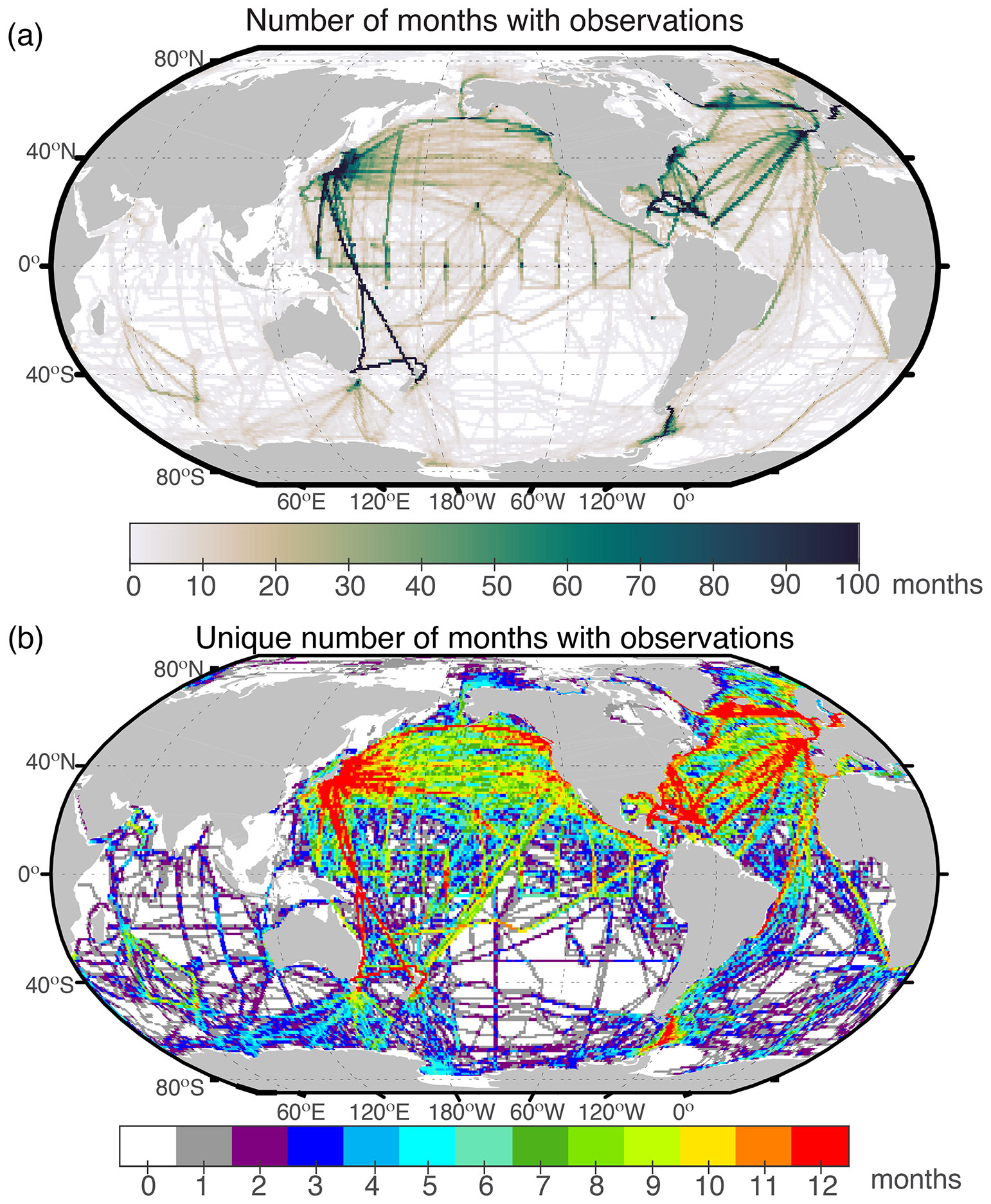
Figure 1(a) Total number of months with at least one observation in each 1° grid cell in the SOCATv2022 database for years 1980–2021 (Bakker et al., 2022). The maximum number possible for a grid cell is 504 (42 years × 12 months). (b) The number of unique calendar months in each grid cell where at least one observation has been made since 1980. Red indicates grid cells where each month (January–December) has been sampled at least once over the (more than) 40-year time series, while white indicates grid cells with no measurements over the length of the time series.

An additional challenge to global monitoring efforts is that observations are not collected consistently throughout the annual cycle in many locations around the globe, thus requiring considerable interpolation to produce a full seasonal climatology. Much of the ocean contains data collected in fewer than three unique months of the year, regardless of how many years of data are available (Fig. 1b). Current efforts utilize proxy variables and machine learning to identify relationships between ocean carbon and better-observed variables (often SST, chlorophyll, mixed layer depth, etc.) and then through those relationships extrapolate available ocean fCO₂ to fill the missing months of the seasonal cycle. Unlike those methods (e.g., methods compared by Rödenbeck et al., 2015), we do not utilize any proxy variables in this method and only rely on available fCO${}_{\mathrm{2}}^{\mathrm{oce}}$ values in the SOCAT database to estimate the seasonal climatology. Hence, this effort provides a complementary alternative interpolation method to other approaches.

2.4 Atmospheric fCO₂

For the calculation of atmospheric carbon dioxide, we utilize zonally invariant NOAA marine boundary layer (MBL) xCO₂ values which are reported in units of ppm or µmol mol⁻¹ (Lan et al., 2023) and provided with each observation in the SOCAT dataset. In order to calculate fCO${}_{\mathrm{2}}^{\mathrm{atm}}$ values from MBL xCO${}_{\mathrm{2}}^{\mathrm{atm}}$ values, we follow standard operating procedures and equations outlined in Dickson et al. (2007) and use the SST, salinity, and sea level pressure observations also reported for each value in the SOCAT database (Bakker et al., 2022). The SST (more specifically ship intake temperature) is measured concurrently with surface ocean CO₂, sea level pressure is from NCEP, and surface salinity is from the World Ocean Atlas (WOA). ΔfCO₂ (ΔfCO₂) is calculated by subtracting corresponding atmospheric values from ocean values ($f{\mathrm{CO}}_{\mathrm{2}}^{\mathrm{oce}}-f{\mathrm{CO}}_{\mathrm{2}}^{\mathrm{atm}}$).

3.1 Normalization to a reference year

In previous versions of the LDEO climatology, emphasis was placed on the calculation of trends in surface ocean carbon levels for all regions of the global ocean. These trends were used to normalize all available observations to one reference year by correcting for the estimated change that would be expected between the collection date of the observation and the reference year. In this updated climatology, we use ΔfCO₂ values as input to the algorithm rather than allowing for the adjustment of fCO${}_{\mathrm{2}}^{\mathrm{oce}}$ to a specific reference year. A similar methodology was used in early versions of the LDEO climatology (i.e., T-1997).

By utilizing this method to collapse all available data to 1 year, we make the assumption (as made by T-1997) that the ocean and atmosphere are changing at the same rate and thus that the ΔfCO₂ has been constant over the (more than) 40 years of observations. This assumption allows for a standard method for the normalization of all observations to 1 calendar year. This method is utilized in contrast to the most recent LDEO climatologies where trends over distinct time periods were investigated and where one trend was then selected for use in time-normalization throughout much of the global ocean (i.e., T-2002, T-2009a, and T-2014).

Atmospheric pCO₂ change drives rising ocean pCO₂, and surface ocean carbon concentrations follow atmospheric increases on multidecadal timescales and over large regions and on the global scale (Fay and McKinley, 2013; McKinley et al., 2020). Large synthesis efforts by those in the global ocean carbon community show that even if ocean trends are larger/smaller than the atmosphere on decadal or multi-year time periods, when considering the longest time periods, the atmosphere and ocean carbon trends are statistically indistinguishable over much of the global ocean (Fay and McKinley, 2013; Tjiputra et al., 2014). While the Tjiputra et al. (2014) and Fay and McKinley (2013) efforts consider large regional analyses, Bates et al. (2014) provide a synthesis of trends in pCO₂ at long-term observing stations, with most of the stations showing a match to the rise in atmospheric CO₂ concentration (Tanhua et al., 2015).

Table S1 in the Supplement shows biome-scale mean fCO₂ trends computed using all available 1° × 1° grid cells with observations in the gridded product released as part of SOCATv2022 (Sabine et al., 2013). We present seasonal trends for each biome due to seasonal sampling bias over much of the global oceans. Similar to T-2009a (see Tables 1–5 of T-2009a), trends for different ocean regions vary significantly (Table S1) due in part to differing years with available data across ocean regions (Fig. S5 in the Supplement). Observations within the Indian Ocean, for example, and other regions with blue shading in Fig. S5 are weighted towards the 1980s and 1990s, while regions stretching across the North Atlantic and North Pacific have been heavily sampled over the last 2 decades with ships of opportunity. These well sampled regions have median years of collected observations later than 2010 (areas with red shading in Fig. S5).

Recent studies (Friedlingstein et al., 2022) demonstrate that, globally, the oceans lag slightly behind the atmosphere in terms of rates of carbon increase; thus, ΔfCO₂ has become increasingly negative as noted above. The central climatological year represented by our method is thus somewhat ambiguous regionally, though globally it is centered at about 2010. The median year of all fCO₂ observations collected in SOCATv2022 greater than 100 km from land is 2013. Since observations are more densely clustered in the recent period, observations in the early period may have a greater weight in determining climatological values. Given global trends, our approach may estimate a smaller ocean sink in regions where the ocean was sampled more heavily early in the time period (e.g., blue shading in Fig. S5) and a greater ocean sink in regions with heavy recent sampling (red shading in Fig. S5). We acknowledge that the assumption of a constant ΔfCO₂ does not take into account the long-term trend in ΔfCO₂; however, our simplified approach avoids application of trends determined for well-observed regions and time periods across poorly observed regions and time periods.

We conducted a sensitivity analysis to demonstrate the impact of the ΔfCO₂ method implemented in this version versus a normalization approach similar to that applied in T-2009a. Specifically, we assumed a homogeneous 1.5 µatm yr⁻¹ trend in fCO${}_{\mathrm{2}}^{\mathrm{oce}}$ for all regions and years and normalized available observations to a reference year of 2010. Spatial maps of the differences in fCO₂ for the year 2010 for the normalization approach versus ΔfCO₂ method are shown in the Supplement (Fig. S6). Globally, the annual ocean uptake created using the 1.5 µatm yr⁻¹ normalization method (T-2009a) is within 3 % of the ΔfCO₂ method (this analysis); specifically, the values are −1.85 Pg C yr⁻¹ versus −1.79 Pg C yr⁻¹ for the 1.5 µatm yr⁻¹ normalization method and the presented ΔfCO₂ approach, respectively, for a reference year of 2010.

3.2 Method for time–space interpolation

The method for spatial interpolation and day of year utilized in the climatology has not changed from the previous versions (e.g., T-2009a). As described above, ΔfCO₂ values are used to compile observations into one reference year in contrast to the time-normalization approach of T-2009a. The spatial interpolation scheme requires that all observations are binned into 4° × 5° grids for each day of the year. In some areas of the global ocean, such as the northern and equatorial ocean regions, there are observations in a majority of the pixels. However, vast expanses in the Southern Hemisphere have few observations in each pixel and there are many pixels that contain no observations at all (Fig. 1).

We follow the same methodology as T-2009a for binning observations in sparsely sampled grid cells south of 12° S. Here, spatial binning is increased by 4 and 5° longitude and latitude, respectively, extending from the center of each grid cell. This creates a grid of overlapping 8° × 10° grid cells. Additionally, bins include the day before and after a given day of year. The mean is computed by weighting measured values inversely proportional to their time–space distance from the pixel center. After the above procedures are applied, more than 50 % of the space–time pixels over the global oceans are filled.

To estimate the ΔfCO₂ values in the remaining cells, an interpolation equation based on the 2-D diffusion–advection transport of surface waters is used, as in T-2009a. The equation is discretized onto a 4° × 5° grid for the global ocean, and it is solved iteratively using a finite difference algorithm (Takahashi et al., 1995; T-1997). The method avoids singularities at the poles by assigning land to each high-latitude region (Antarctica in the south and treating the highest latitudes of the Arctic Ocean as land in the north). With this method, the resulting ΔfCO₂ values are the solutions obtained after 500 iterations, as previously determined on the basis of interpolation experiments of temperature values (T-2009a).

With this interpolation scheme, observed ΔfCO₂ values where available are preserved, and the continuity equation is used to compute values for grid cells that have no observations. Consistent with previous iterations of this approach, the combined effects of internal sources and sinks of carbon, CO₂ exchange with the atmosphere, and upwelling of deep waters are all assumed to be included in the analysis of the observations that feed into the interpolation scheme. Uncertainties persist due to the sparsity of input data, normalization to a reference year, and the space–time interpolation. In part to address these uncertainties, we report only monthly means.

To maintain consistency with similar products and input datasets for flux calculations, we downscale to 1° boxes by assigning all twenty 1° × 1° pixels in a 4° × 5° grid cell the same ΔfCO₂ value. When calculating sea–air fluxes, because the other inputs to the flux calculation such as wind speed are varying on a 1° × 1° resolution grid, differences in the gridded flux climatology emerge on this finer spatial scale.

3.3 Flux calculation method: pySeaFlux

To assess the near-global ocean carbon sink associated with these ΔfCO₂ estimates, air–sea CO₂ exchange must be calculated. The gridded monthly 1° × 1° ΔfCO₂ values were used to compute air–sea CO₂ fluxes using the bulk formulation with Python package pySeaFlux v1.3.1 (https://github.com/lukegre/SeaFlux, last access: 1 June 2023; Gregor and Fay, 2021). The net sea–air CO₂ flux (F) is estimated using

where kw is the gas transfer velocity, sol is the solubility of CO₂ in seawater (in units of mol m⁻³ µatm⁻¹), fCO${}_{\mathrm{2}}^{\mathrm{oce}}$ is the partial pressure of carbon in the surface ocean (in µatm), and fCO${}_{\mathrm{2}}^{\mathrm{atm}}$ (in units of µatm) represents the atmospheric CO₂ levels in the marine boundary layer. Finally, to account for the seasonal ice cover at high latitudes, the fluxes are weighted by one minus the ice fraction (ice), i.e., the open ocean fraction. By utilizing the pySeaFlux package (Fay et al., 2021; Gregor and Fay, 2021), we are able to include multiple scaled gas transfer velocities for three different wind products, and our resulting flux estimate is a mean of the three. Additional inputs to the flux calculation include EN4.2.2 salinity (Good et al., 2013), SST and ice fraction from NOAA Optimum Interpolation Sea Surface Temperature V2 (OISSTv2; Reynolds et al., 2002), and European Centre for Medium-Range Weather Forecasts (ECMWF) ERA5 sea level pressure (Hersbach et al., 2023). Finally, surface winds and the associated wind scaling factor for the Cross-Calibrated Multi-Platform v2 (CCMP2; Atlas et al., 2011), the Japanese 55-year Reanalysis (JRA-55; Kobayashi et al., 2015), and the ECMWF ERA5 (Hersbach et al., 2023) reanalysis products are used.

Fluxes reported here use inputs from the year 2010 for the kw, sol, and ice fraction variables. Alternatively, we have calculated fluxes using a mean over a 17-year time period centered on the year 2010. This yields a very similar value with the mean difference being a 0.04 Pg C yr⁻¹ increase in estimated carbon uptake.

4.1 Climatological mean distribution of surface water ΔfCO₂

4.1.1 Global

The near-global 12-month climatological mean distribution of ΔfCO₂ (fCO${}_{\mathrm{2}}^{\mathrm{oce}}$ minus fCO${}_{\mathrm{2}}^{\mathrm{air}}$) is reported for the SOCAT database (Fig. 2; Fay et al., 2023). Evident in the mapped climatology are the large-scale patterns across the global ocean: the consistent high (positive) ΔfCO₂ values in the equatorial Pacific region where upwelling is a dominant influence and low (negative) values of ΔfCO₂ in the North Atlantic region where evaporation leads to increased salinity and cooling, driving strong uptake of carbon and subduction of surface waters.

A near-global mean climatology curve shows a bimodal shape in ΔfCO₂, with a smaller peak in boreal spring (March/April) and a much larger peak in late boreal summer (August/September), clearly driven by the hemispheric seasonal cycles (Fig. 2a). The global curve reaches its minimum in November and begins a recovery throughout the boreal winter before dipping again to a springtime minimum in June. The near-global annual mean ΔfCO₂ value is −4.1 µatm (with temporal standard deviation equal to 1.6 µatm), and it is notable that the global mean ΔfCO₂ value is below zero for every month of the year, suggesting that seasonally the global ocean mean is a perpetual carbon sink with expansive regions of uptake nearly always outweighing smaller regions of efflux (Figs. 2, 3). On the other hand, the northern and southern hemispheric seasonal cycles each exhibit peaks in ΔfCO₂ above zero during their corresponding warm/summer months (Fig. 2a).

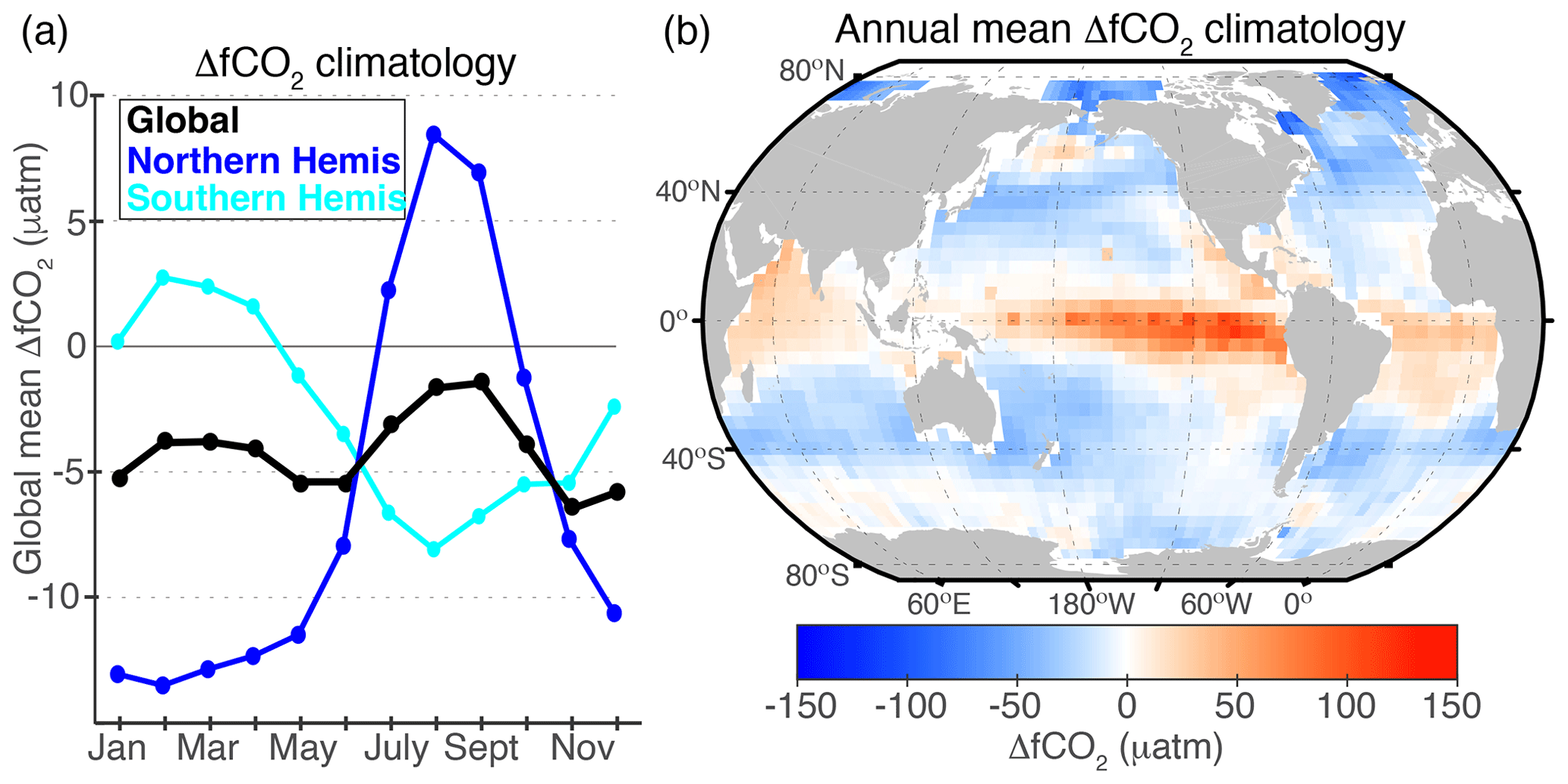
Figure 2(a) Global mean and Northern Hemisphere and Southern Hemisphere ΔfCO₂ seasonal climatology from the SOCAT database. (b) Map of annual ΔfCO₂ climatology.

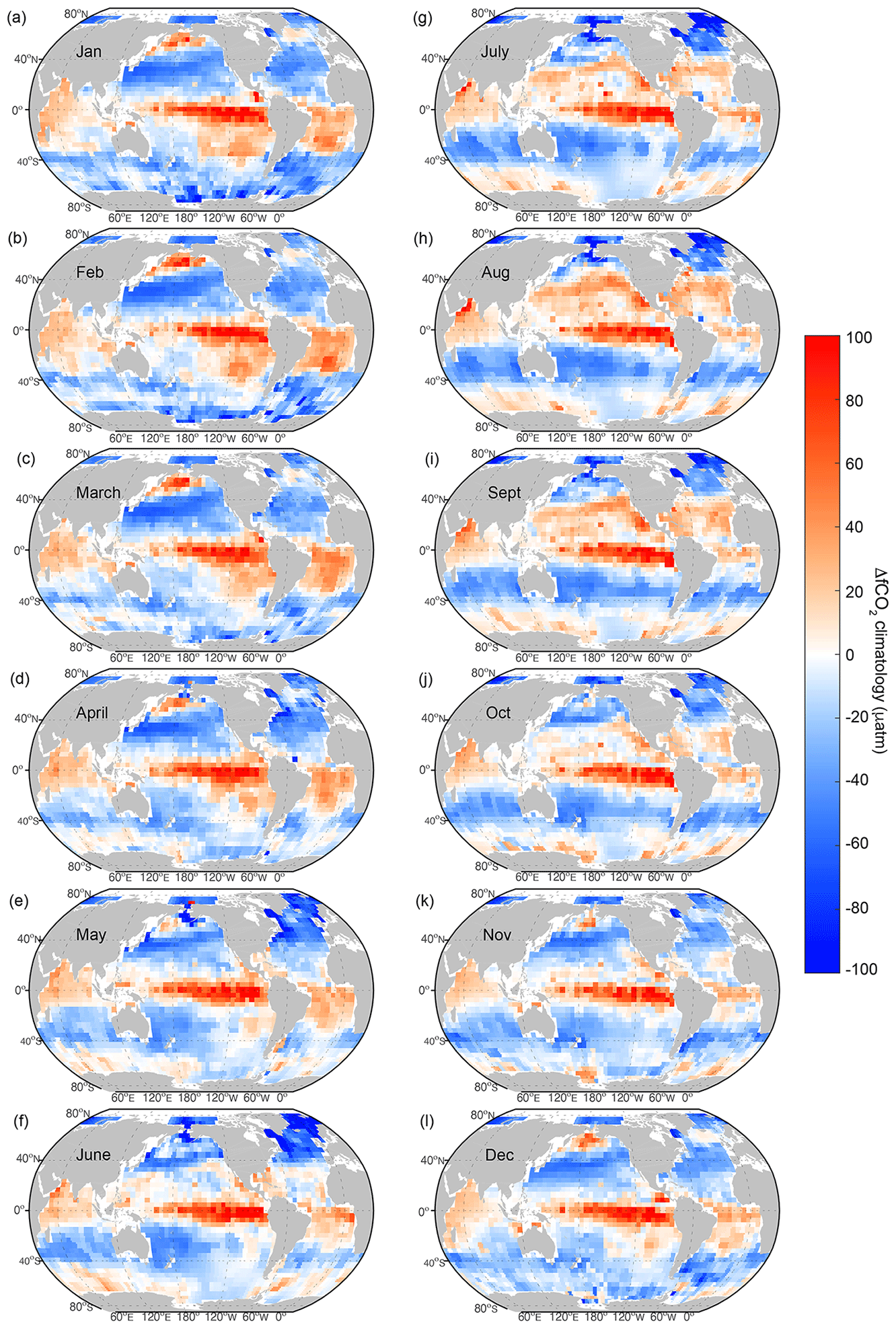
Figure 3Monthly mean values for sea–air ΔfCO₂. Warm colors indicate positive ΔfCO₂ (ocean is greater than atmospheric CO₂), white indicates near zero ΔfCO₂, and cool colors indicate negative ΔfCO₂ (ocean CO₂ is lower than the atmosphere).

4.1.2 Regional

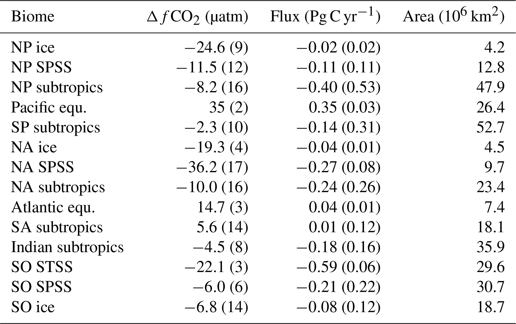
To show the seasonal changes in ΔfCO₂ more clearly, it is valuable to consider the patterns exhibited over consistent biogeochemical regions around the globe. For this analysis, we utilize the biomes of Fay and McKinley (2014), but for simplicity we combine the seasonally stratified and permanently stratified subtropical biomes into one region in the Northern Hemisphere (referred to simply as subtropical in this article). Monthly climatologies for each of the biomes are shown (Fig. 4) in addition to the grid-scale maps for each climatological month which allows for further regional interpretation (Fig. 3). Table 1 lists the annual mean ΔfCO₂ values in each of these regions.

Figure 4Monthly climatology of ΔfCO₂ for each regional ocean biome in the (a) Atlantic, (b) Pacific, and (c) Indian and Southern Ocean basins. (d) Map of regional biomes. Colors of curves correspond to regions on the map in panel (d), with labels in matching colored text. Note that the y axis varies between subplots. Values for each region's annual mean and standard deviations are listed in Table 1.

The equatorial regions of the Pacific and Atlantic oceans have positive ΔfCO₂ values throughout the annual cycle and little seasonal variability. This indicates that the area is a source of CO₂ to the atmosphere year round. The equatorial Pacific (Fig. 4b) has the highest positive ΔfCO₂ values (annual mean = 35.4 µatm), followed by the tropical Atlantic (Fig. 4a; annual mean = 14.8 µatm).

The subtropical biomes, representing the temperate North and South Atlantic and Pacific basins exhibit large seasonal ΔfCO₂ cycles which change sign throughout the year. Here, the ΔfCO₂ cycle is largely temperature driven. Positive ΔfCO₂ in warm summer months and negative values in colder winter months, reflecting the dominance of seasonal temperature changes on the cycles of ocean fCO₂ in these regions. The seasonal amplitude for the subtropical North Pacific is 44.7 µatm, and it is slightly larger than the seasonal amplitude in the subtropical North Atlantic (42.7 µatm). Since the mean seasonal amplitudes for SST are quite similar in these two ocean basins, with the Atlantic having a slightly larger seasonal change in surface temperature (4.4 °C in Pacific and 5.0 °C in Atlantic; not shown), the difference in ΔfCO₂ amplitudes between the Pacific and Atlantic subtropical regions cannot be attributed solely to SST, and it may reflect differences in biogeochemical cycling between these two basins.

Seasonal changes in the northern subtropical oceans are roughly 6 months out of phase from the southern subtropical biomes. The South Pacific subtropical biome has a seasonal amplitude of 29.8 µatm which is nearly 15 µatm smaller than that of the North Pacific subtropical biome. In contrast, the seasonal amplitude of the South Atlantic subtropical basin is just 1 µatm smaller than its counterpart in the North Atlantic (the South Atlantic subtropical amplitude is 41.7 µatm). The Indian Ocean subtropical biome which encompasses most of the Indian Ocean, both above and below the Equator, has a smaller ΔfCO₂ amplitude (22.3 µatm), but the phasing matches well with both the South Pacific and South Atlantic subtropical biomes, with peak (positive) ΔfCO₂ values in February and the lowest values in August. The smaller ΔfCO₂ seasonal amplitudes in the Indian and South Pacific subtropical basins are partially attributable to lower SST variability in these regions (SST seasonal cycle amplitudes are 4.0 and 3.0 °C in the South Pacific and Indian subtropics, respectively, compared to 4.6 °C in the subtropical South Atlantic). However, it is likely that both differences in spatiotemporal patterns of primary productivity and undersampling in the South Pacific and Indian subtropics (Fig. 1) also contribute to differences in ΔfCO₂ seasonal amplitudes between these basins.

The timing of the ΔfCO₂ trough in the subpolar regions is opposite that of the subtropical North Pacific and Atlantic basins. Strongly negative ΔfCO₂ in the spring and summer months is due to the effects of intense biological drawdown which quickly and dramatically lowers carbon levels in the subpolar surface ocean with the onset of the growing season. Biological productivity and strong spring/summer stratification result in subpolar seasonal cycles that are roughly 4 to 6 months out of phase compared to adjacent subtropical regions. In the Atlantic subpolar biome, ΔfCO₂ values are consistently below zero throughout the annual cycle (a maximum of −15.1 µatm occurs in February). In the subpolar North Pacific basin, positive ΔfCO₂ values are present over the boreal winter (January–March) before biological drawdown associated with the spring bloom lowers the ΔfCO₂ values back below zero for the remainder of the year. The spring drawdown is weaker in the subpolar North Pacific compared to the subpolar North Atlantic.

Figure 4c displays the seasonal cycle for the Southern Ocean biomes including the seasonal ice biome, the subpolar region, and the seasonally stratified subtropical region of the Southern Hemisphere. The higher latitude subtropical region has negative ΔfCO₂ values throughout the year and a relatively small seasonal ΔfCO₂ amplitude compared to the more expansive South Atlantic, South Pacific and Indian subtropical basins to the north. The mean ΔfCO₂ and seasonal amplitude for the Southern Ocean subtropical region is −22.5 and 9.0 µatm, respectively.

The Southern Ocean subpolar and ice biomes both have relatively strong seasonal cycles, reaching maximums of ΔfCO₂ near and slightly above zero, respectively, during the late austral winter and early austral spring (Fig. 4c). This positive peak during July through October in the Southern Ocean seasonal ice zone is influenced by under-ice vertical mixing with deep waters that contain excess carbon and nutrients. During the austral spring and summer months, intense phytoplankton blooms occur near and around the edges of the retreating sea ice in the seasonal ice zone and within the subpolar region. These blooms cause dramatic drops in ΔfCO₂ values at the end of the calendar year (October–December). Limited sampling and smoothing from the interpolation method fail to capture the high spatiotemporal variability that characterizes this highly dynamic region.

Table 1Mean annual fCO₂ and flux in global open ocean biomes (Fay and McKinley, 2014). Value in parentheses is 1 standard deviation over the 12-month climatology. Area of each biome is also included. NP: North Pacific; SP: South Pacific; NA: North Atlantic; SA: South Atlantic; SO: Southern Ocean. SPSS: subpolar seasonally stratified; STSS: subtropical seasonally stratified. Northern Hemisphere subtropical regions are reported to match the regions shown in Fig. 4 (combining the permanently and seasonally stratified subtropical biomes from Fay and McKinley, 2014, into one).

Download Print Version | Download XLSX

4.2 Net air–sea CO₂ flux

The mean climatological global air–sea CO₂ flux estimate using the SOCAT database is −1.79 Pg C yr⁻¹, indicating uptake of carbon by the ocean. This is a slightly greater flux into the ocean than the direct estimate from the previous version of the climatology (T-2009a), which reported a direct estimated global mean flux of −1.4 Pg C yr⁻¹ for the year 2000. For the uncertainty in global ocean–atmosphere CO₂ flux, we use the methods described in T-2009a with updated uncertainty estimates as reported when applicable. Wanninkhof et al. (2013) followed the same approach as T-2009a with consideration of updated synthesis work (Ho et al., 2011). Our approach combines uncertainty contributions from the spatial (13 % or ±0.23 Pg C yr⁻¹; T-2009a) and temporal (±0.5 Pg C yr⁻¹; T-2009a) sampling of ΔfCO₂ as well as smaller contributions for the uncertainty in the gas exchange parameterization (20 % or ±0.36 Pg C yr⁻¹; Wanninkhof, 2014), wind (±0.09 Pg C yr⁻¹; Fay et al., 2021), and riverine carbon (±0.2 Pg C yr⁻¹; Jacobson et al., 2007). This yields an uncertainty estimate of ±0.7 Pg C yr⁻¹ (when summed in quadrature) on our mean climatological global air–sea CO₂ flux estimate.

Results discussing the net flux produced from the LDEO pCO₂ database climatology are included in the Supplement.

4.2.1 Mean annual distribution

The near-global mean flux estimate presented here represents 90 % of the surface area of the global ocean. Specifically, this estimate excludes the coastal ocean and areas of the high-latitude seas. We have chosen to present the near-global flux value discussed above without any adjustment which could account for missing areas. Suggested methods for filling missing ocean areas in such reconstructions are available in Fay et al. (2021) but are not implemented in this climatology to remain consistent with its previous versions. An estimate of the flux from regions missing from this product can be obtained by using the full-coverage pCO₂ climatology combining open and coastal oceans (Landschützer et al., 2020). Considering only grid cells in the Landschützer et al. (2020) product that are missing in this climatology, we estimate an annual average coastal and high-latitude flux of −0.38 Pg C yr⁻¹. The flux adjustment for missing areas of this climatology varies throughout the seasonal cycle, ranging from −0.43 to −0.31 Pg C yr⁻¹ during the 12 months of the climatology. This quantity is not included in the climatological estimate presented here.

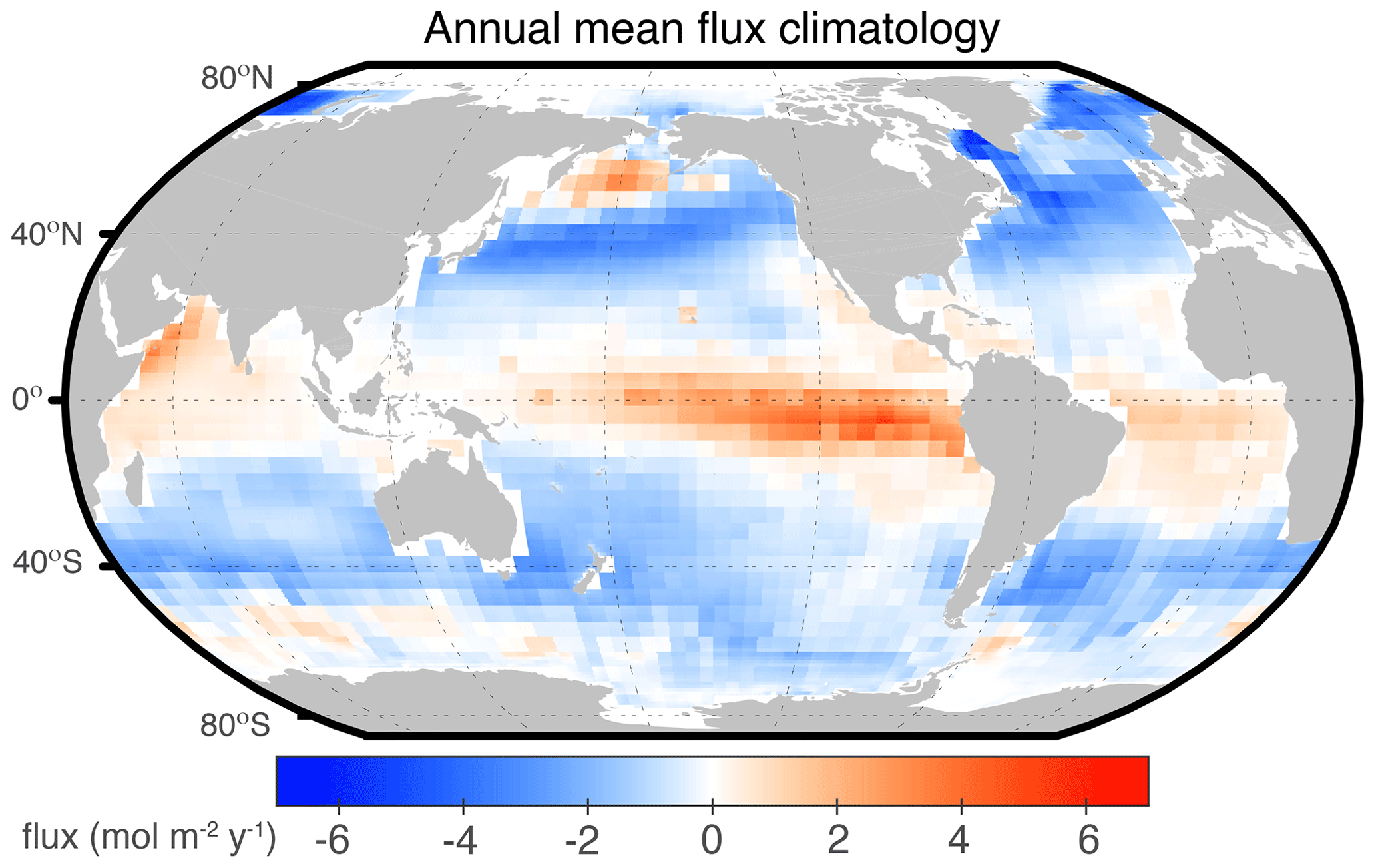
Figure 5Annual mean CO₂ flux calculated from the SOCAT database. Flux is calculated using the SeaFlux method using the mean of three wind speed reanalysis products. Warm and cool colors indicate regions of carbon efflux and uptake, respectively. The near-global mean flux is −1.79 Pg C yr⁻¹.

Figure 5 shows the climatological mean annual sea–air CO₂ flux (mol m⁻² yr⁻¹) and maps of two seasons (DJF and JJA) are displayed in Fig. 6. Annual mean sea–air CO₂ flux values for the ocean regions are summarized in Table 1. The equatorial Pacific is the most prominent atmospheric CO₂ source region, with a seasonally persistent sea-to-air flux of 0.35 Pg C yr⁻¹. When combined with the equatorial Atlantic region, the tropical belt emits an annual mean of 0.39 Pg C yr⁻¹ to the atmosphere. Adjacent to this tropical efflux zone are vast expanses of seasonally variable flux patterns. The subtropical basins in both hemispheres act as CO₂ sinks in the cooler months and transition to regions of neutral or small CO₂ sources during the warmer months. At higher subtropical latitudes, strong winds and relatively low ocean fCO₂ values occur along the subtropical convergence zone where the cooled subtropical gyre waters with low fCO₂ values meet the subpolar waters with biologically lowered fCO₂.

The Northern Hemisphere mid- and high-latitude regions represent a smaller sink compared to the corresponding regions of the Southern Hemisphere (Table 1), largely due to the overall greater surface area of the oceans in the Southern Hemisphere (oceans south of 35° S are 25 % of total global ocean area, while oceans north of 35° N are 15 % of total ocean area). The dramatic influence of the expansive Southern Hemisphere oceans is also demonstrated by the large flux in the Southern Ocean subtropical region (−0.59 Pg C yr⁻¹) that represents 8 % of the global ocean surface area.

Moving poleward, a strong sink (−0.27 Pg C yr⁻¹) occurs in the North Atlantic subpolar region which includes the Nordic Seas and the portions of the Arctic Ocean which contain observations. This strong localized carbon sink is attributed to the import of low anthropogenic waters at depth in the Gulf Stream that are exposed as mixed layers deepen (Ridge and McKinley, 2020) and to large phytoplankton blooms in spring followed by cooling in winter. In the Southern Ocean, annual mean CO₂ flux is heterogeneous and relatively small in the seasonal ice zone due to the ice cover that reduces sea–air gas transfer in winter. Additionally, the small annual flux values in the Southern Ocean subpolar and ice regions (−0.21 and −0.08 Pg C yr⁻¹, respectively) are a result of a cancellation of the seasonal source (winter) and sink (summer) fluxes.

4.2.2 Seasonal variation of sea–air CO₂ flux

Seasonal variations in air–sea fluxes are clearly seen in the climatology (Fig. 6) and are attributed to a combination of effects including fluctuations in SSTs, biological uptake of carbon dioxide, and mixing and wind speeds.

The seasonal variability of fluxes in higher latitudes of the subtropics in the Atlantic, Indian, and Pacific oceans cause an oscillation from neutral or weak sources of CO₂ to the atmosphere in the warmer seasons to strong CO₂ sinks in the cooler or winter seasons. Water cools as it is transported poleward by western boundary currents, allowing for carbon uptake (Ayers and Lozier, 2012). In spring and summer, the biological drawdown of carbon increases CO₂ uptake by the ocean, partially offset by increases in fCO₂ due to warming.

Subtropical gyre regions also transition from weak sinks in the winter seasons to weak sources in the summer seasons, following the seasonal SST cycles and reflecting the dominance of temperature effects in controlling the seasonal variability in the fCO₂ and sea–air fluxes in oligotrophic gyres. In tropical low-latitude regions, seasonality is generally smaller; however, localized hot spots of high variability and large fluxes do exist, such as in the northwestern Indian Ocean where the strong summer monsoon winds force upwelling of carbon-rich subsurface waters and cause high gas transfer rates in this region (Chen and Tsunogai, 2019; T-2002; Sabine et al., 2000). The equatorial Pacific and Atlantic show little seasonal variability in CO₂ flux with a persistent efflux throughout the year.

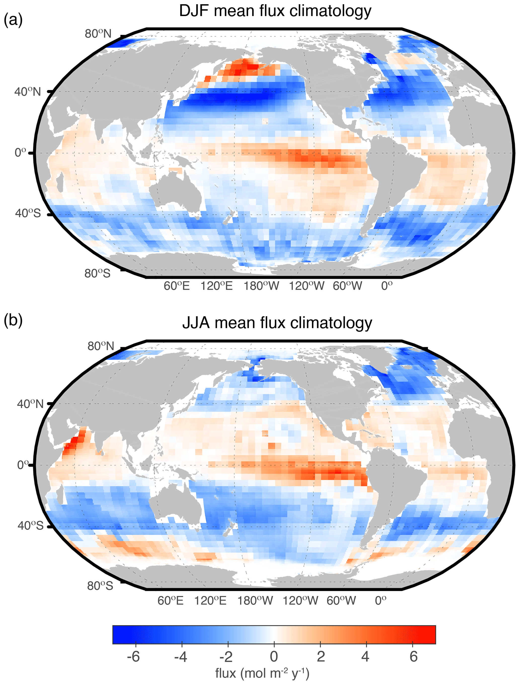
Figure 6Season sea–air CO₂ flux (mol C m⁻² yr⁻¹) climatology for (a) December–January–February (DJF) and (b) June–July–August (JJA). Positive values (warm colors) indicate sea-to-air fluxes (ocean efflux), and negative values (cool colors) indicate air-to-sea fluxes (ocean uptake).

In the Southern Ocean, there is a consistent region of moderate carbon source waters located in the Atlantic and Indian Ocean sector south of 45° S latitude during the austral winter (Fig. 6b). The source in the Southern Ocean region could be influenced by high fCO₂ waters from margins of the Antarctic sea-ice field given that the efflux values occur during the austral winter months (JJA). As the seasons transition to warmer temperatures and the ice edge recedes, this region is impacted by high rates of photosynthesis, causing fCO₂ drawdown and resulting in a transition to moderate carbon sinks during the austral summer (DJF). Another possibility is that the austral winter carbon source is linked to deep mixing and/or upwelling water which would bring an import of high dissolved inorganic carbon (DIC) to the surface layers. Given the limited number of observations, particularly in winter in the Southern Ocean (Fig. 1), confidence in the resulting climatology is lower in this region.

5.1 Comparison with the T-2009a climatology

In the previous release of this climatology (T-2009a), pCO₂ values were corrected to a reference year of 2000 using a mean atmospheric CO₂ increase rate of 1.5 µatm yr⁻¹ over the entire ocean area with the exception of the Bering Sea, where the observed rate of −1.2 µatm yr⁻¹ was used. In our updated method described above (Sect. 3.1), we eliminate the need to apply a normalization rate for observations and instead calculate a ΔfCO₂ value for each observation using a colocated concurrent atmospheric fCO₂ value. We note that T-2014 presents a more updated pCO₂ climatology than T-2009a. Since T-2014 emphasizes climatologies for the other carbonate system variables (pH, dissolved inorganic carbon, and total alkalinity) and omits estimation of fluxes, we focus our comparison on values presented in T-2009a.

Spatial differences between the climatology created from surface water ΔfCO₂ values using the methods discussed above and the approach of T-2009a (3 million observations) are shown in Fig. 7 for the months of February and August – months were selected for consistency with past comparisons presented in T-2009a and T-2002. The differences between this updated release and previous versions producing climatologies for reference years 2000 (T-2009a) and 1990 (T-1997) are unlikely to represent real change in the oceans over time, but they instead primarily reflect the impact of the greatly expanded database as well as the use of the ΔfCO₂ approach as opposed to the time-normalization method of T-2009a (Fig. S9).

The most significant regional differences between this updated version and that of T-2009a are observed over the subpolar North Atlantic, the subtropical Southeast Pacific, and portions of the Southern Ocean. In the North Atlantic, differences between versions are largest in the boreal winter (February map, top panel of Fig. 7) when the updated climatology exhibits less uptake compared to the T-2009a version (positive values on the map indicate more negative values in the T-2009a version). Differences in the North Atlantic can be at least partially attributed to the much greater availability of observations in this region between the two databases (Figs. 1, S1, S9). This is discussed in further detail in the Supplement text.

The Southeast Pacific is an area with very limited observations, but a few key datasets have been included in the SOCAT database since 2010. Figure 1 shows that despite these recent additions to SOCAT, there are still only a few observations covering this region. Comparison of Fig. 3 in this study with Fig. 9 of T-2009a suggests that the additional datasets in SOCATv2022 result in a more defined seasonal cycle for fCO₂ in the subtropical Southeast Pacific in the current release. Specifically, the map of differences shown in Fig. 7 shows that this region is a greater source of carbon to the atmosphere in austral summer and a greater sink in austral winter compared to T-2009a (compare also Fig. 6 of this study with Fig. 15 of T-2009a). In contrast, monthly maps included in Fig. 3 of T-2009a show little seasonal contrast in ΔpCO₂ likely due to a lack of observations.

In the Southern Ocean region during austral winter (August), ΔfCO₂ values are more negative in the current version compared to T-2009a. The Southern Ocean is also a region of limited data availability, particularly in austral winter, but one where SOCATv2022 also includes several datasets added in the past decade that have an outsized influence on the resulting climatology.

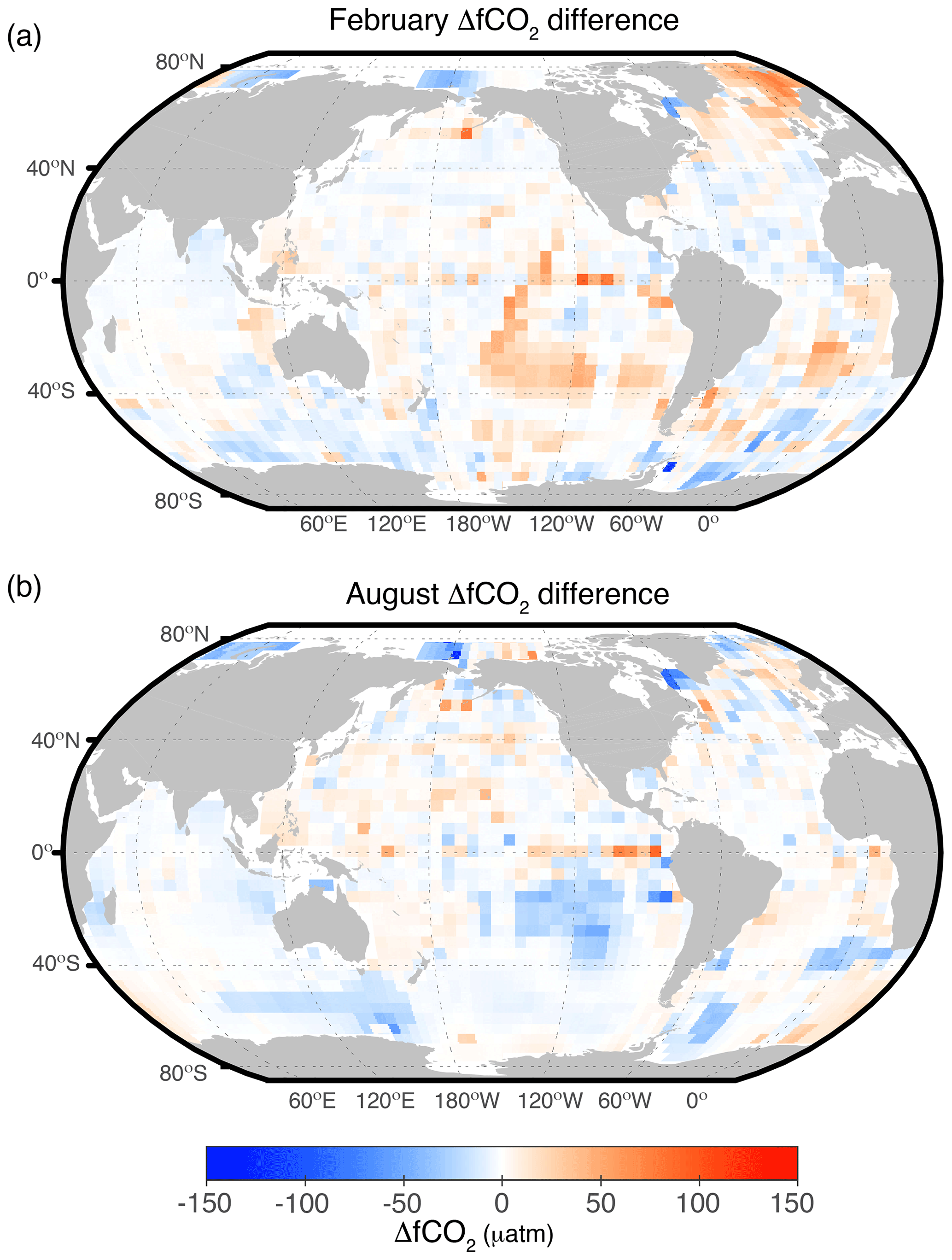
Figure 7Difference maps for the surface water ΔfCO₂ climatology produced by this study using SOCAT and that from T-2009a (maps show this study minus T-2009a) in (a) February and (b) August. In T-2009a, the ΔCO₂ values are reported as pCO₂, and here we are using fCO₂.

5.2 Comparison to other flux estimates

The estimate presented here for annual global mean carbon flux (−1.79 Pg C yr⁻¹) represents slightly less uptake than reported by other studies, but given uncertainties, as well as differing time frames, spatial coverage, and gap-filling methodologies, our estimate compares closely with current estimates similarly based on observed surface ocean fCO₂.

To compare our new climatological estimate of contemporary air–sea net flux from surface ocean fCO₂ with estimates of the anthropogenic carbon flux from interior data (e.g., Gruber et al., 2019) or estimates from global ocean biogeochemical models (e.g., Friedlingstein et al., 2022; Hauck et al., 2020), it is necessary to account for the outgassing of natural carbon supplied to the ocean by rivers. This riverine estimate varies significantly in magnitude between studies and continues to be a research focus for the ocean carbon community. Therefore, we focus on comparisons between our climatological estimate and a mean carbon flux estimate from an ensemble of observation-based pCO₂ products included in the SeaFlux product (Fay et al., 2021).

The SeaFlux products span the years 1985–2020, are all similarly based on the SOCAT database, but employ various methods of machine learning and interpolation to produce full-coverage ocean carbon maps. For this comparison, a climatology of the SeaFlux product is produced, and fluxes are calculated in the same manner as for the climatology presented here. Following this approach, the SeaFlux climatology ensemble yields a global mean flux of −2.10 Pg C yr⁻¹, which represents a slightly larger flux into the ocean than that produced by the updated climatology ($-\mathrm{1.79}\pm \mathrm{0.7}$ Pg C yr⁻¹). The differences in global flux can be attributed to the true global coverage of the SeaFlux product relative to the 90 % global ocean coverage of this study. As mentioned above in Sect. 4.2, an estimate of missing coastal and high-latitude fluxes increases the ocean carbon uptake estimate for this climatology by roughly 0.38 Pg C yr⁻¹. Adding this additional flux brings our analysis within 0.1 Pg C yr⁻¹ of the SeaFlux ensemble (−2.17 versus −2.10 Pg C yr⁻¹ for this analysis versus the SeaFlux estimate, respectively).

Spatially, comparison of the SeaFlux ensemble of products to our climatology shows strong agreement in overall patterns but significant differences in the mid- and high-latitude Southern Hemisphere oceans (Fig. 8). Gloege et al. (2021) analyzed a machine learning method's ability to reconstruct global carbon fluxes from available observations using a test-bed approach and found the highest flux bias in the Southern Ocean regions as well as an overestimation of decadal variability in this region. Given the limited availability of year-round observations at high Southern Hemisphere latitudes, and the resulting reliance on various gap-filling approaches, it is not surprising that the largest differences between the climatology presented here and the SeaFlux ensemble emerges in this region. Significant differences between these climatologies are also evident in the high latitude North Pacific and North Atlantic, specifically in the boreal winter season (Fig. 8a). Again, a lack of observations in these regions during the winter season (Fig. 1) likely accounts for much of this disagreement, with more reliance on the interpolation methods used by each method. Machine learning methods that utilize proxy variables to estimate pCO₂ in unsampled areas, such as those in the SeaFlux product, often rely on relationships derived from better-observed areas that are deemed similar in biogeochemical characteristics and it is likely that the mechanisms at these high-latitude locations are not accurately captured by any available interpolation methods. This is also a current focus of research for the ocean-carbon-observing community.

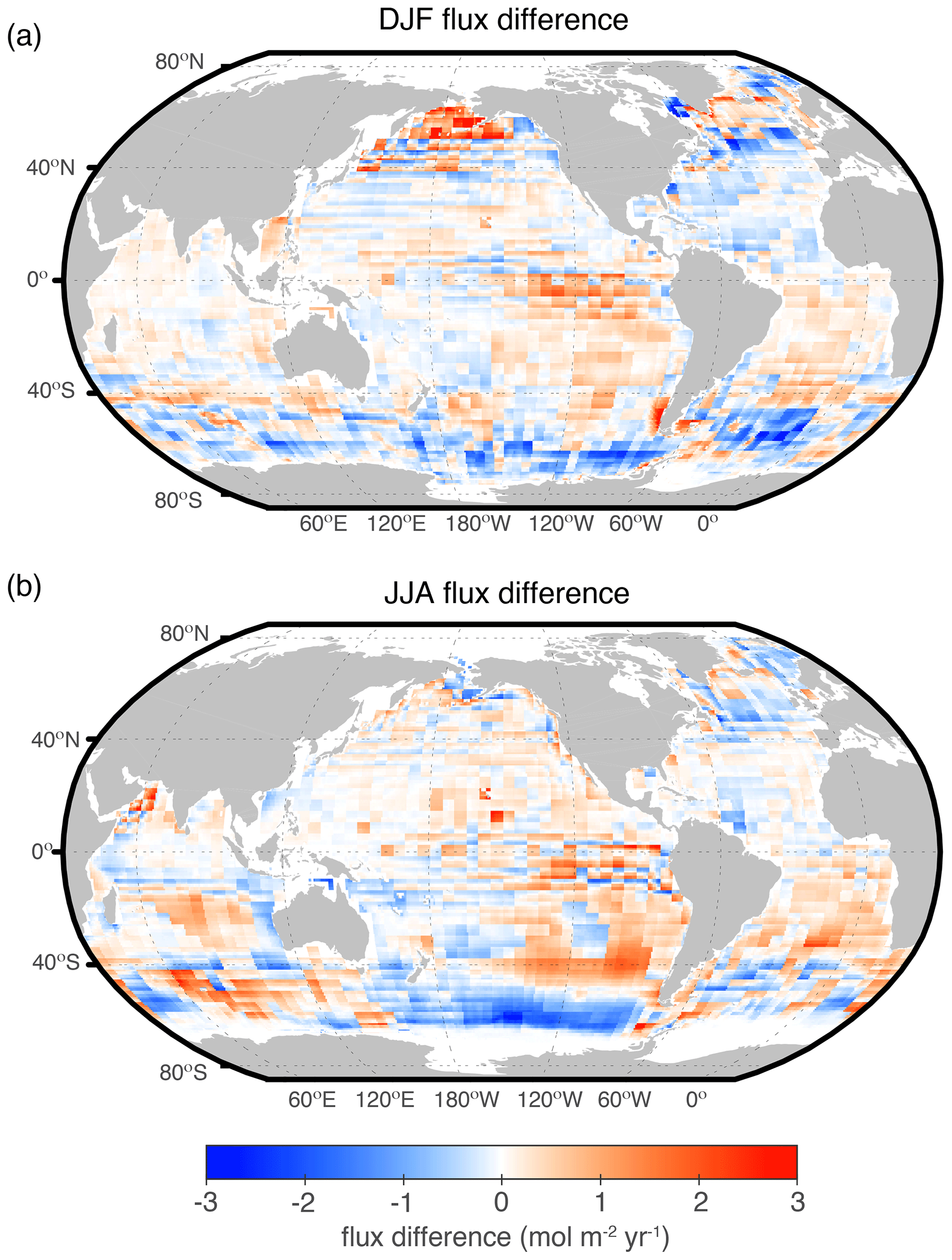
Figure 8Difference map for carbon fluxes (mol m⁻² yr⁻¹) calculated from this ΔfCO₂ climatology and fluxes reported by an ensemble of observation-based products included in the SeaFlux product for (a) boreal winter, DJF, and (b) boreal summer, JJA. Map shows the difference defined as this study minus SeaFlux. Note that white areas at the poles are due to ice coverage extent (and therefore no value reported in the climatology) and not a flux difference of zero.