

Abstract
We present an inference method utilizing artificial neural networks for parameter estimation of a quantum probe monitored through a single continuous measurement. Unlike existing approaches focusing on the diffusive signals generated by continuous weak measurements, our method harnesses quantum correlations in discrete photon-counting data characterized by quantum jumps. We benchmark the precision of this method against Bayesian inference, which is optimal in the sense of information retrieval. By using numerical experiments on a two-level quantum system, we demonstrate that our approach can achieve a similar optimal performance as Bayesian inference, while drastically reducing computational costs. Additionally, the method exhibits robustness against the presence of imperfections in both measurement and training data. This approach offers a promising and computationally efficient tool for quantum parameter estimation with photon-counting data, relevant for applications such as quantum sensing or quantum imaging, as well as robust calibration tasks in laboratory-based settings.
Export citation and abstract BibTeX RIS

Original content from this work may be used under the terms of the Creative Commons Attribution 4.0 license. Any further distribution of this work must maintain attribution to the author(s) and the title of the work, journal citation and DOI.
1. Introduction
Quantum parameter estimation refers to the fundamental problem of inferring the value of unknown physical quantities within a quantum system [1]. It has important practical applications in device characterization [2–4], quantum feedback and control [5–10] and quantum communications [11, 12], and most importantly, it is at the core of the field of quantum metrology [13–21], whereby quantum correlations are exploited to estimate physical quantities with high precision.
The most conventional approach to quantum parameter estimation is based on the following steps: (i) prepare a quantum system in a given state; (ii) allow it to evolve through a unitary transformation that encodes the unknown parameters; (iii) perform a measurement on the system; (iv) estimate the parameter from the measurement results; (v) repeat the process to gather statistical information and increase the precision of the estimation [15, 17]. Beyond this standard prepare-evolve-measure approach, there are relevant situations where, instead, one performs a single-shot continuous quantum measurement on a quantum probe [1]. In this case, one is interested in obtaining an estimation that will be continuously updated as data is gathered over the time evolution of a single quantum trajectory. Protocols of quantum parameter estimation from continuous measurements have been developed and studied over the years [22–35]; such parameter estimation techniques are particularly relevant for applications such as atomic magnetometry [36–38], quantum metrology with open quantum systems [28, 39–41] or estimation of classical time-dependent signals [42]. Previous works have established computational approaches to calculate the probability density  [23, 29–32] of unknown n-dimensional parameters
 ![$\theta = [\theta_1,\theta_2,\ldots,\theta_n]$](https://content.cld.iop.org/journals/2058-9565/9/3/035018/revision2/qstad3c68ieqn2.gif) conditioned on the continuously recorded data, D, which could correspond, for instance, to photon-counting records [30, 31, 43], continuous weak measurements [44–46], or homodyne measurements [32]. These calculations rely on the application of Bayes' theorem on the likelihood functions
conditioned on the continuously recorded data, D, which could correspond, for instance, to photon-counting records [30, 31, 43], continuous weak measurements [44–46], or homodyne measurements [32]. These calculations rely on the application of Bayes' theorem on the likelihood functions  , obtained as the trace of un-normalized conditional density matrices with the evolution conditioned on the measured data record [47].
This Bayesian approach provides, in principle, the most accurate description of the knowledge that can be gained about θ given the measurement data D. However, the application of this technique faces several difficulties. Firstly, it requires exact modelling of the open quantum system and any source of error, which can become challenging for noisy, complex quantum systems [48]. Secondly, the method can be computationally demanding. For instance, when tackling the problem of multi-parameter estimation, where one wishes to estimate several parameters simultaneously, Bayesian inference calls for the use of stochastic methods to sample the posterior probability distribution [29]. Generally, the Bayesian parameter estimation method will be computationally time-consuming, even in simple systems. This hampers the prospects for real-time estimation and for the integration of the inference process in the actual measurement device taking the data, which would be desirable for reduced latency and energy consumption [49, 50].
A novel approach to this problem that has gained attention in recent years is the application of machine-learning methods in which a neural network (NN) is trained to aid in the inference process. Crucially, this method allows to circumvent the requirement for detailed knowledge of the underlying physical system, as long as a reasonable amount of training data is available. The use of NNs have been demonstrated for a variety of tasks in quantum metrology, including parameter estimation in the presence of unavoidable noise [51–55], calibration [56, 57], phase estimation in interferometry [56–58], magnetometry [55, 59], control [54], and tomography [60, 61]. In the context of continuously monitored systems, NNs have been employed for the reconstruction of quantum dynamics [2, 62] and parameter estimation under continuous weak dispersive measurements [51, 52, 59, 63], which are characterized by a continuous, diffusive evolution of the quantum system [1, 64].
Here, we assess the potential of deep learning to tackle the parameter estimation task from continuous measurements of the photon-counting type. These measurements are described by point processes that, rather than yielding a diffusive evolution of the system, are characterized by sudden quantum jumps upon the acquisition of a discrete signal, such as the detection of a single photon [1]. This type of measurements, ubiquitous in the field of quantum optics and cavity-QED [65–72], provide insights into the particle-like nature of quantum systems and can produce strongly correlated signals that directly violate classical inequalities, as in the case of the renowned effect of photon antibunching [72]. Our work addresses the question of whether NNs can effectively process and exploit the quantum correlations present in this type of discrete signals.
Our proposed NN architectures approach this task as a regression problem, taking the time delays between individual photodetection events as an input and providing an estimate  for the desired parameters of interest as the output, as sketched in figure 1. Our main finding is that the NNs can take advantage of the quantum correlations within the signal, providing higher precision than using an equivalent signal that lacks these correlations, e.g. the integrated intensity value. By computing the root-mean-squared error (RMSE) of the estimations, we find that, after training, the NN can reach the limit of precision established by Bayesian inference, while requiring dramatically fewer computational resources. We also demonstrate that parameter estimation with NNs could be more resilient to noise than a simple Bayesian approach with no detailed knowledge of the underlying noise sources incorporated into the model, since it is possible for NNs to indirectly learn the noise model during the training phase. In contrast to a full Bayesian posterior distribution, the architectures studied in this work provide a single point estimate of the parameters, without including a confidence interval. Nevertheless, we evaluate their efficiency as estimators by conducting statistical analyses of their performance across numerous data samples.

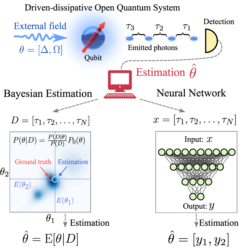
Figure 1. Quantum parameter estimation strategies in open quantum systems. Parameters are encoded in the dynamics of an open quantum system: here, these are the frequency detuning between the qubit transition frequency and the drive frequency,  , and the Rabi frequency Ω of the coherent drive, proportional to the dipole moment of the qubit and the amplitude of the electromagnetic field driving it. Photon-counting measurements of the quantum light radiated yield a record of the times of photodetection. The unknown parameters can be reconstructed through Bayesian parameter estimation (left). Here, we show the posterior probability distribution
  for the data obtained from a single quantum trajectory, from which an estimator
  is obtained by computing the mean value of the distribution. The ground truth value for the parameters is contained within the posterior distribution in a region of high probability. An alternative approach is based on the use of neural networks (right). The neural network learns the inverse process that maps observed data to the parameters
  through an initial training phase that employs data generated with known parameters. Once trained, inference for new data is much faster using the neural network than repeating the Bayesian parameter estimation with the new data.
Download figure:
Standard image High-resolution image2. System and data generation
The data we use to train the deep NNs and perform parameter inference consists of simulated measurements of single photo-detection times from the light emitted by a driven two-level system (TLS). This system represents a paradigmatic example of the types of quantum parameter estimation problems studied extensively in the literature [22, 23, 28]. It is a prototypical model that can describe various quantum emitters, such as quantum dots [73], molecules [74], or color centres [75]. We consider a TLS with states  , lowering operator
  and transition frequency ωq
, continuously excited by a coherent drive with frequency ωL
and a Rabi frequency Ω. This quantum probe is coupled to the environment, giving rise to spontaneous emission with a rate γ. In the frame rotating at the drive frequency, the dynamics of such a system is described by the master equation (we set
and transition frequency ωq
, continuously excited by a coherent drive with frequency ωL
and a Rabi frequency Ω. This quantum probe is coupled to the environment, giving rise to spontaneous emission with a rate γ. In the frame rotating at the drive frequency, the dynamics of such a system is described by the master equation (we set  herein):

where  and
and ![$D(\hat x)[\hat\rho]\equiv 2 \hat x \hat\rho \hat x^\dagger - \left\{\hat x^\dagger \hat x,\hat\rho \right\}$](https://content.cld.iop.org/journals/2058-9565/9/3/035018/revision2/qstad3c68ieqn13.gif) follows the definition of the Lindblad superoperator [76]. The interplay between continuous driving and losses eventually brings the system into a steady state.
follows the definition of the Lindblad superoperator [76]. The interplay between continuous driving and losses eventually brings the system into a steady state.
The estimation is performed using the data D generated by the continuous photon-counting measurement of the radiation emitted by the system during a single run of the experiment, considering an initial state  and a total evolution time, T, much longer than the relaxation time towards the steady state. We simulate this process using the Monte Carlo method of quantum trajectories [1, 47, 77] implemented in the QuTiP library [78, 79]. Under continuous photon-counting measurements, the system evolves stochastically under the following rules:
- at every differential time step,
 , the system can experience a quantum jump with a probability , which corresponds to the detection of a photon emitted by the system;
 - otherwise, the system follows a non-Hermitian evolution . The wavefunction is normalized in each time step.


![$|\psi(t+\textrm{d}t)\rangle \propto [\mathbf{I}-i(\hat H - i \hat\sigma^\dagger\hat\sigma/2)\textrm{d}t]|\psi(t)\rangle$](https://content.cld.iop.org/journals/2058-9565/9/3/035018/revision2/qstad3c68ieqn18.gif)
Each stochastic simulation of a trajectory corresponds to an individual realization of the experiment, generating a data vector by storing the specific set of times  when a photodetection leading to a quantum jump occurs during the course of a total evolution time T, with N being the total number of jumps recorded. For convenience, we define our data as the set of time delays between these jumps,
 ![$D = [\tau_1,\ldots,\tau_N]$](https://content.cld.iop.org/journals/2058-9565/9/3/035018/revision2/qstad3c68ieqn20.gif) , where
, where  ,
,  and t0 = 0 (see appendix
  after each emission [30].
Each trajectory is simulated for an evolution time T chosen to generate a data record D of precisely N = 48 jumps. This number is chosen to meet a compromise; it is sufficiently large to ensure that the system is in a steady state, while also allowing for inference with a limited number of photons in a relatively short timescale spanning just a few tens of emitter lifetimes, which is typically within the range of nanoseconds for solid-state quantum emitters [66]. It is important to note that fixing N requires that each trajectory will have a different evolution time T [80, 81]. While the choice of fixing N allows us to work straightforwardly with inputs of uniform dimension, there may be experimental scenarios where T is a more relevant metrological resource. In such cases, it may be necessary to maintain a fixed T while allowing N to vary. Even in this scenario, the analysis outlined below remains applicable, and the design and training of the NNs could be easily adapted, as we discuss in appendix
After obtaining the data D from a single trajectory or experiment, our goal is to estimate the unknown parameters θ that govern the dynamics of the system. In this study, we specifically focus on the parameters Δ and/or Ω, considering that γ is known. While this might be an idealized setting, it is instructive enough to benchmark the power of quantum correlations and NNs for the task of parameter estimation. We are interested in benchmarking the NNs against the ultimate precision limit set by the Bayesian inference process. This process yields a posterior probability distribution for the unknown parameters conditioned on the measured data D: following Bayes' rule we have  . A comprehensive explanation of Bayesian inference from continuous measurements is provided in [28] and, within the context of this work, in appendix
 ![$\theta = [\Delta]$](https://content.cld.iop.org/journals/2058-9565/9/3/035018/revision2/qstad3c68ieqn37.gif) , in the top panel, and the TLS population in the bottom panel. Red grid lines mark the times when a quantum jump takes place. One can see how the regions of high probability in the posterior distribution concentrate more around the ground truth as time increases and more data is collected.
, in the top panel, and the TLS population in the bottom panel. Red grid lines mark the times when a quantum jump takes place. One can see how the regions of high probability in the posterior distribution concentrate more around the ground truth as time increases and more data is collected.

Figure 2. Classical and quantum data. (a) Dynamics of an individual Monte Carlo quantum jump trajectory for  . Top panel shows the posterior probability of the parameter Δ for the photon-counting data D(t) acquired up to time t from a certain trajectory, starting from a flat prior. Bottom panel shows the corresponding evolution of the population of the qubit for the same trajectory, with red grid lines marking the times when a quantum jump occurs, leading to the collapse of the population to zero and subsequently restarting the system from the
  state. The list of time delays between jumps constitutes the quantum data D from which we infer the unknown parameters θ. (b) Waiting-time distribution
  of the measured time delays τi
between photo-detection events during an individual trajectory, which constitute the quantum signal. The plot shows the distribution for several Δ parameters of the system. Clear patters emerge which are Δ-dependent. A classical signal corresponding to the integrated intensity is defined as the mean of the measured delays,
of the measured time delays τi
between photo-detection events during an individual trajectory, which constitute the quantum signal. The plot shows the distribution for several Δ parameters of the system. Clear patters emerge which are Δ-dependent. A classical signal corresponding to the integrated intensity is defined as the mean of the measured delays,  . Since all τi
are independent random variables coming from the same underlying distribution
. Since all τi
are independent random variables coming from the same underlying distribution  ,
, ![$\mathrm{E}[\bar\tau] = \mathrm{E}[\tau_i] = \mathrm{E}[\tau]$](https://content.cld.iop.org/journals/2058-9565/9/3/035018/revision2/qstad3c68ieqn29.gif) , shown as a black-dashed line. The red vertical gridline marks the value
, shown as a black-dashed line. The red vertical gridline marks the value  used as ground truth in panel (a). The horizontal grid line marks the corresponding expected value
 $](https://content.cld.iop.org/journals/2058-9565/9/3/035018/revision2/qstad3c68ieqn31.gif) (c) Heatmap of normalized histograms of τ obtained from 104 trajectories with N = 48 clicks each, simulated with
(c) Heatmap of normalized histograms of τ obtained from 104 trajectories with N = 48 clicks each, simulated with  . The oscillatory patterns of the waiting-time distribution are clearly reproduced in the histograms, which represent the quantum data. (d) Histogram of all the values
  obtained for the 104 trajectories used in panel (c). This represents the classical data, given by the mean of delays measured in a given trajectory. The resulting Gaussian distribution is centered around
 ![$\mathrm{E}[\tau]$](https://content.cld.iop.org/journals/2058-9565/9/3/035018/revision2/qstad3c68ieqn34.gif) , marked by the dashed red gridline. We fix
, marked by the dashed red gridline. We fix  in all panels. All units are defined in terms of γ.
Download figure:
Standard image High-resolution imageOnce the posterior distribution is obtained, we build an estimator by taking the mean, ![$\hat\theta = \textrm{E}[\theta|D] = \int \textrm{d}\theta P(\theta|D)\theta$](https://content.cld.iop.org/journals/2058-9565/9/3/035018/revision2/qstad3c68ieqn38.gif) , which is known to be the estimator that minimizes the RMSE [83]. While reducing the full posterior to a single estimation
, which is known to be the estimator that minimizes the RMSE [83]. While reducing the full posterior to a single estimation  implies a loss of information and involves a subtle choice of the best estimator, this step allows us to straightforwardly compare the result with the estimation provided by the NNs. Here we also note that we use a flat (uniform) prior on the parameters of interest, while in general the Bayesian framework allows us to introduce our knowledge of the system using arbitrary priors.
A central question of our study is whether NNs can leverage the quantum correlations in the data. The emission from a TLS is strongly correlated; the fact that the emitter can only store one excitation at a time gives rise to the well-known non-classical phenomenon of antibunching [72], i.e. the suppressed probability of detecting two photons simultaneously. These quantum correlations can be evidenced through several observables, such as the waiting-time distribution  (the probability of two consecutive emissions to be separated by a time delay τ), which presents a vanishing value at zero delay,
  , and an oscillatory behaviour that depends strongly on the system parameters. These features, shown in figure 2(b), are translated directly into the histograms of time delays observed in each individual trajectory, as we show in figure 2(c). We will refer to a signal containing these time delays as a quantum signal.
To assess the information contained in these correlations, we compare it to an equivalent classical signal where the only relevant value is the integrated intensity, i.e. the total number of counts detected per unit time,  . We can interpret such a classical signal as measurements lacking the necessary time resolution to detect individual photons, providing an integrated intensity without any access to the internal temporal correlations between photon emissions. In fact, we choose the inverse of the intensity as the classical signal, since it conveniently represents that we have reduced the list of measured delays, that constitute the quantum signal, by taking their average,
  . Since
  is a sum or independent random variables τi
that all follow the probability distribution
is a sum or independent random variables τi
that all follow the probability distribution  , the central limit theorem ensures that, when N is large,
  is itself a random variable that follows instead a normal distribution, with
 ![$\text{E}[\bar\tau] = \text{E}[\tau_i]$](https://content.cld.iop.org/journals/2058-9565/9/3/035018/revision2/qstad3c68ieqn47.gif) . This normal distribution stands in contrast to the more complicated probability distribution
. This normal distribution stands in contrast to the more complicated probability distribution  followed by the individual random variables τi
. In the steady state, this distribution is centered around
followed by the individual random variables τi
. In the steady state, this distribution is centered around ![$\text{E}[\tau_i] = \text{E}[\tau]\equiv\int \textrm{d}\tau w(\tau)\tau = (\langle\hat\sigma^\dagger\hat\sigma\rangle_\mathrm{ss} \gamma)^{-1}$](https://content.cld.iop.org/journals/2058-9565/9/3/035018/revision2/qstad3c68ieqn49.gif) (see figure 2(d)).
(see figure 2(d)).
Access to ![$\text{E}[\tau]$](https://content.cld.iop.org/journals/2058-9565/9/3/035018/revision2/qstad3c68ieqn50.gif) instead of
instead of  represents an obvious loss of information, where any contributions from quantum correlations is completely discarded. Thanks to this, the RMSE of the estimation made by using the classical signal serves as a reference for comparison when doing estimations with the full quantum signal: whenever the obtained RMSE is lower than that of the classical signal, we understand that the estimation method is taking some advantage from quantum correlations. The process of parameter estimation from this classical signal, described in more detail in appendix
  is the mean of the posterior
  .
.
3. Training
We considered different neural-network architectures with the common structure of inputs and outputs that we illustrate in figure 1. The input consists of a vector ![$ x = D = [\tau_1, \tau_2, \ldots, \tau_N]$](https://content.cld.iop.org/journals/2058-9565/9/3/035018/revision2/qstad3c68ieqn54.gif) of time delays between photodetection events, while the output is a vector of size n corresponding to the estimations of the n-dimensional estimation problem,
of time delays between photodetection events, while the output is a vector of size n corresponding to the estimations of the n-dimensional estimation problem, ![$ y = [\hat\theta_1, \hat\theta_1, \ldots, \hat\theta_n]$](https://content.cld.iop.org/journals/2058-9565/9/3/035018/revision2/qstad3c68ieqn55.gif) . Here, we treat both one-dimensional estimation problems, with
. Here, we treat both one-dimensional estimation problems, with ![$\theta = [\Delta]$](https://content.cld.iop.org/journals/2058-9565/9/3/035018/revision2/qstad3c68ieqn56.gif) in the 1D case, and
in the 1D case, and ![$\theta = [\Delta, \Omega]$](https://content.cld.iop.org/journals/2058-9565/9/3/035018/revision2/qstad3c68ieqn57.gif) in the 2D case. We fixed the size of the input vector to N = 48, indicating that our networks perform estimations based on a single experiment run once 48 photons have been detected.
in the 2D case. We fixed the size of the input vector to N = 48, indicating that our networks perform estimations based on a single experiment run once 48 photons have been detected.
Estimation via NNs requires a training stage akin to a calibration process (learning phase). In this work, the input data used for training,  , consists of a list of time delays obtained from trajectories simulated in QuTiP, with the corresponding target data
  being the ground truth parameters used to run the simulations. Our best results are achieved using two types of architectures:
- 1.RNN: recurrent neural network (RNN) with two long short-term memory (LSTM) layers. These networks can learn correlations in sequential data, rendering them particularly promising for exploiting temporal quantum correlations. It is worth noting that there are no such correlations between time delays in our present system, since the τi are independent due to the collapse following a quantum jump. Nonetheless, these networks still deliver a very good performance. More information on these networks and their application in parameter estimation from continuous signals can be found in [59].
- 2.Hist-Dense: Fully connected NN with a first custom layer designed to return a histogram of the input data. The geometry of the bins of the histogram is defined by the number of bins and their range. We set these as non-trainable hyperparameters fixed at 700 total bins and a range given by and . This layer produces an efficient, physically-informed representation of the data, which leverages the absence of correlations between time delays in this particular system.


Further details on the networks and the training process, can be found in appendix  (which we assume to be a known parameter) by fixing γ = 1. After training, we benchmark the estimations made by the NNs against the estimation made through Bayesian inference and, in the single-parameter estimation case, also against the estimation done on the classical version of the signal. Details of this validation process are in appendix
4. Single-parameter estimation (1D)
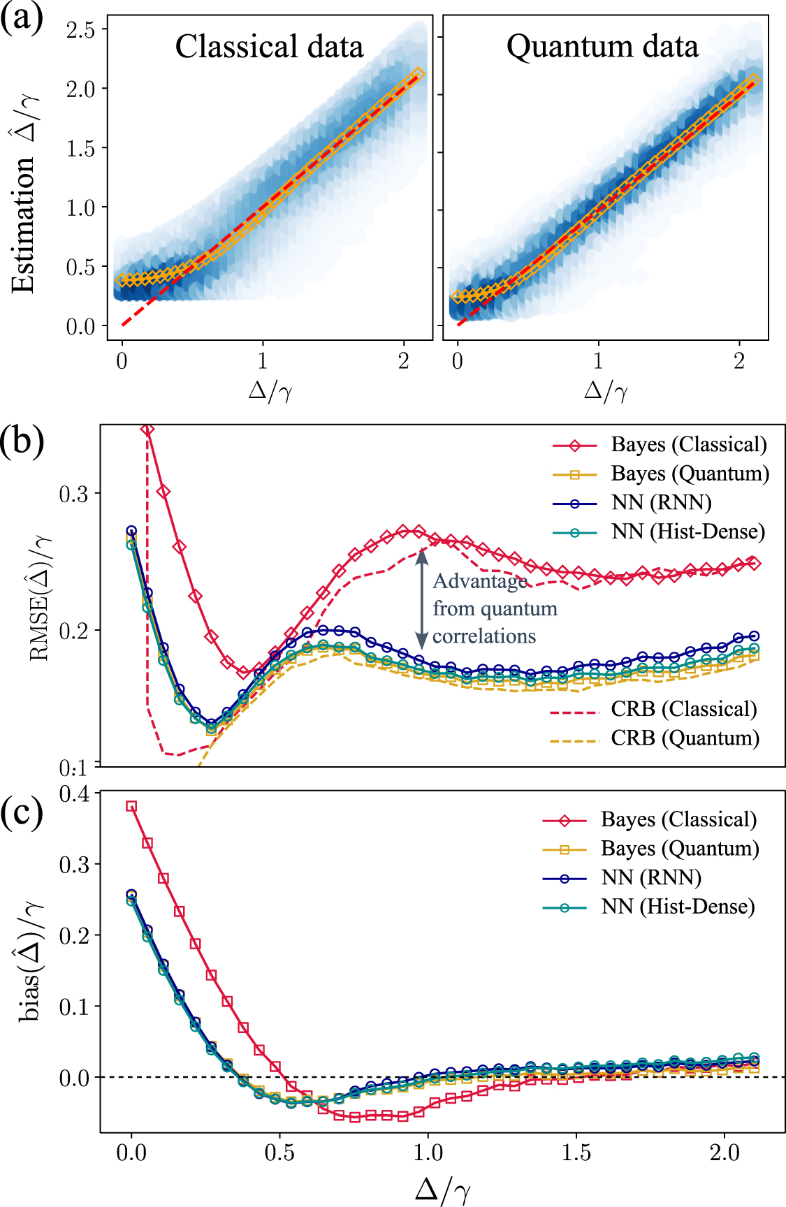
First, we focus on the simplest situation in which a single parameter is estimated: the detuning ![$\theta = [\Delta]$](https://content.cld.iop.org/journals/2058-9565/9/3/035018/revision2/qstad3c68ieqn63.gif) . Figure 3(a) depicts a scatter plot of the predictions made by each method for different values of Δ. These plots show that the predictions made using the quantum signal—regardless of whether Bayesian inference or NNs are used—are more densely concentrated around the ground truth than the predictions obtained using the classical version of the signal. This already suggests that quantum correlations in the data can provide an advantage.
. Figure 3(a) depicts a scatter plot of the predictions made by each method for different values of Δ. These plots show that the predictions made using the quantum signal—regardless of whether Bayesian inference or NNs are used—are more densely concentrated around the ground truth than the predictions obtained using the classical version of the signal. This already suggests that quantum correlations in the data can provide an advantage.

Figure 3. Performance of different estimation strategies. (a) Scatter plot of estimations  across a range of Δ values from classical (left) and quantum (right) versions of the photon-counting signal, computed for 104 trajectories for each Δ value. All the different estimators used for quantum data (Bayesian, NN) give a similar result, so only one is shown (NN-Hist). The blue shade of the points represents the underlying probability density function obtained through kernel density estimation. The dashed red line represents the ground truth. Orange points represent the mean of the the estimations. (b) RMSE of the estimators for on classical (red) and quantum (yellow, blue, green) versions of the signal. Estimations on quantum signals clearly outperform the classical estimation, signaling the useful information encoded in quantum correlations. The predictions made by NNs (blue, green) are on par with Bayesian inference (yellow), which is the optimal process in terms of information retrieval. Dashed lines mark the lower limit set by the biased Cramér-Rao bound for the classical and quantum signals. (c) Bias of the predictions for the same cases as in (b).
Download figure:
Standard image High-resolution image
This advantage is clearly quantified in figure 3(b), which compares the RMSE of the predictions obtained by each of the methods computed on a different set of validation trajectories (see appendix
We note, however, that none of the approaches studied here provided an estimator that is unbiased for all Δ, as we show in figure 3(c). There, we plot the bias of several estimators, defined as  . This bias is not problematic per se, since it is known that biased estimators can be preferable to unbiased ones in some cases [83]. However, this bias needs to be taken into account at the time of comparing the obtained RMSE with the lower bound set by the Fisher information and the Cramér–Rao bound (CRB) [84, 85]. As we discuss in more detail in [82], one needs to consider the biased CRBs [86]. We calculated the Fisher information and the biased CRBs for the photon-counting measurements considered here [28–30], incorporating the calculated biases shown in figure 3(c). The resulting lower limits for the RMSE are shown as dashed lines in figure 3(b). We show that, for the quantum signal, both the Bayesian and NN estimators saturate the CRB for a wide range of values of Δ.
5. Multi-parameter estimation (2D)
We also benchmarked our results for the 2D parameter-estimation case, where both Δ and Ω are unknown and estimated simultaneously, ![$\theta = [\Delta,\Omega]$](https://content.cld.iop.org/journals/2058-9565/9/3/035018/revision2/qstad3c68ieqn66.gif) .
.
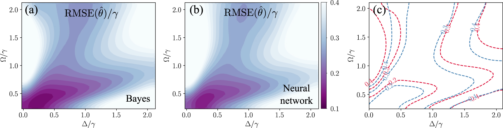
Our results for the 2D estimation case are shown in figure 4. In panel (a), we depict the RMSE of Bayesian estimation from the quantum signal in a region of the plane ![$[\Delta,\Omega]$](https://content.cld.iop.org/journals/2058-9565/9/3/035018/revision2/qstad3c68ieqn67.gif) . The resulting map shows a nontrivial structure that reflects the underlying physical complexity of the system and that is consistent with previous reports in the literature [29, 30]. The same physical complexity is captured by the NNs, as shown in figure 4(b), which depicts the RMSE obtained by the estimation of a Hist-Dense architecture and shows that the RMSE reflects the same underlying structure as the one obtained with Bayesian inference, yielding comparably small values overall. Both results can be more clearly compared in figure 4(c), depicting overlaying contour lines of the two plots in panels (a) and (b).
. The resulting map shows a nontrivial structure that reflects the underlying physical complexity of the system and that is consistent with previous reports in the literature [29, 30]. The same physical complexity is captured by the NNs, as shown in figure 4(b), which depicts the RMSE obtained by the estimation of a Hist-Dense architecture and shows that the RMSE reflects the same underlying structure as the one obtained with Bayesian inference, yielding comparably small values overall. Both results can be more clearly compared in figure 4(c), depicting overlaying contour lines of the two plots in panels (a) and (b).

Figure 4. Multidimensional parameter estimation for ![$\theta = [\Delta, \Omega]$](https://content.cld.iop.org/journals/2058-9565/9/3/035018/revision2/qstad3c68ieqn68.gif) . The qubit-drive detuning Δ and the Rabi frequency Ω are estimated simultaneously. (a) RMSE of the estimations made through Bayesian inference. (b) RMSE of the estimations made by the NN. (c) Contours corresponding to Bayesian (red) and NN (blue) are overlaid for the sake of comparison.
. The qubit-drive detuning Δ and the Rabi frequency Ω are estimated simultaneously. (a) RMSE of the estimations made through Bayesian inference. (b) RMSE of the estimations made by the NN. (c) Contours corresponding to Bayesian (red) and NN (blue) are overlaid for the sake of comparison.
Download figure:
Standard image High-resolution imageOur results clearly establish that NNs are able to exploit the information hidden in quantum correlations in order to perform parameter estimation. Given their comparable precision to Bayesian inference, a careful evaluation of the benefits of opting for NNs as an alternative becomes important.
6. Computation efficiency
A first aspect in which NNs can bring an important advantage is the efficiency of the computation, which is particularly relevant for the case in which one wishes to achieve real-time estimation. For the 2D case of simultaneous estimation of two parameters, the posterior for a single trajectory for Bayesian estimation can be computed using the UltraNest package [87] (see appendix
7. The challenge of noise
Another important challenge faced by the Bayesian inference approach is the requirement of a precise modelling of the underlying physical system. This become particularly problematic in the presence of noise, which not only requires a perfect characterization and modelling of the different sources of imperfections, but also makes the subsequent calculation of posteriors much more involved. In contrast, the model-agnostic approach of using NNs allows for a robust prediction without the need of any modelling of the sources of noise, only by training the network directly on noisy data. In the particular case of photon-counting with single-photon detectors, numerous sources of noise can be attributed just to the detection process, such as the efficiency, bandwidth, dead time, dark counts or jitter noise [71]. All these sources of noise have non-trivial consequences on the statistics of the photodetection events [88] and on the quantum trajectories associated to these imperfect measurements [89]. Hence, the necessity of a perfect modelling and characterization of these processes seriously hampers the utilization of Bayesian inference.
7.1. Noise in x: time jitter
We illustrate the potential advantage brought in by the estimation with NNs by considering the particular case of time jitter [88], which we describe by adding a noise term to the values of time delays τ used both in the training and estimation of the NNs for the 1D estimation case ![$\theta = [\Delta]$](https://content.cld.iop.org/journals/2058-9565/9/3/035018/revision2/qstad3c68ieqn69.gif) . We consider noise following a normal distribution with standard deviation στ
, so that
. We consider noise following a normal distribution with standard deviation στ
, so that  , with
  . In order to assess the resilience of the NN predictors to this type of noise, we defined a list of values of στ
in the range
. In order to assess the resilience of the NN predictors to this type of noise, we defined a list of values of στ
in the range ![$\sigma_\tau\in[0,\gamma^{-1}]$](https://content.cld.iop.org/journals/2058-9565/9/3/035018/revision2/qstad3c68ieqn72.gif) . For each value in this list, we sampled a population of
. For each value in this list, we sampled a population of  and trained a model with the corresponding noisy data.
The resulting RMSE of the predictions returned by each of these models is computed using the same validation trajectories used in figure 3, but containing an added Gaussian noise with the same στ as the data used to train the model. The resulting RMSEs are shown in figure 5(a), compared to the RMSE of the prediction via an imperfect Bayesian inference process in which the noise is not explicitly modeled. We observe that, in the case of NNs, the results are more insensitive to the jitter noise and the RMSE of the NN predictor is always lower than that of the Bayesian predictor. This result remains true for all values of Δ, as shown in figure 5(b). We emphasize that this did not require any modelling of the imperfections, as would have been required for a correct process of Bayesian inference. The latter would presumably recover the values reported by the NN, but requiring a perfect characterization of the sources of noise, which may be challenging in some scenarios.

Figure 5. Parameter estimation with noisy data. (a) RMSE of NN predictor trained and evaluated with data containing jitter noise given by a Gaussian distribution with standard deviation στ
(green circles). This is compared to the RMSE of Bayesian inference lacking a description of the noise (yellow crosses). Results shown for a fixed  . (b) Same as in panel (a), shown versus Δ and with a fixed jitter noise
  . RMSE of Bayesian predictor in the absence of noise shown for comparison (gray crosses). (c) RMSE of NN predictor trained with noisy target training data
  , with noise following a Gaussian distribution with standard deviation σy
. We observe that the RMSE of the NN predictor (green circles) can remain smaller than the standard deviation of the training data σy
(gray dot-dashed line). The horizontal grid line marks the RMSE of Bayesian inference with noiseless data for comparison . Results shown for a fixed
, with noise following a Gaussian distribution with standard deviation σy
. We observe that the RMSE of the NN predictor (green circles) can remain smaller than the standard deviation of the training data σy
(gray dot-dashed line). The horizontal grid line marks the RMSE of Bayesian inference with noiseless data for comparison . Results shown for a fixed  . (d) Same RMSE as in panel (c), shown as a function of Δ. Different colors represent different values of σy
, which are also represented as horizontal grid lines, confirming that the RMSE of NN predictor remains smaller than σy
for all values of Δ.
. (d) Same RMSE as in panel (c), shown as a function of Δ. Different colors represent different values of σy
, which are also represented as horizontal grid lines, confirming that the RMSE of NN predictor remains smaller than σy
for all values of Δ.
Download figure:
Standard image High-resolution image7.2. Noise in : imperfect calibration

Another relevant question is the effect of noise in the training target data  . In particular, we consider the case in which the target data used for training differs from the underlying ground truth used to generate the quantum trajectories by a Gaussian noise term with standard deviation σy
, so that
. In particular, we consider the case in which the target data used for training differs from the underlying ground truth used to generate the quantum trajectories by a Gaussian noise term with standard deviation σy
, so that  , with
  . This could reflect, for instance, the finite precision of a calibration device employed to experimentally measure the set of target values used to train the network.
The question we address is whether a NN will be able to perform parameter estimation with a lower RMSE than the standard deviation σy
of the noisy target data used for training. A positive answer to this question would indicate that the precision of the NN estimator can outperform that of the calibration method or device used to generate the training data. Figures 5(c) and (d) illustrate that this scenario is indeed possible. Similarly to the process described for figure 5(a), we defined a series of values of σy
and, for each value, we sampled a population of  and trained a model with noisy target data. The validation of the trained models is done using the same set of trajectories as in figure 3. Figure 5(c) shows that, once the standard deviation of the noisy training target data σy
(dot-dashed line) becomes greater than the RMSE achievable in the noiseless case (horizontal grid line), the predictions made by the NNs trained with this noisy data remain robust and approximately equal to the ideal RMSE. As σy
increases, the RMSE of the NN predictor eventually reaches a threshold where it starts increasing as well, but remaining much smaller than σy
. Such threshold is established by the size of the training dataset. This observation holds for all values of Δ, as shown in figure 5(d). This result highlights the potential of the NNs to improve sub-optimal estimations used to feed the training process.
and trained a model with noisy target data. The validation of the trained models is done using the same set of trajectories as in figure 3. Figure 5(c) shows that, once the standard deviation of the noisy training target data σy
(dot-dashed line) becomes greater than the RMSE achievable in the noiseless case (horizontal grid line), the predictions made by the NNs trained with this noisy data remain robust and approximately equal to the ideal RMSE. As σy
increases, the RMSE of the NN predictor eventually reaches a threshold where it starts increasing as well, but remaining much smaller than σy
. Such threshold is established by the size of the training dataset. This observation holds for all values of Δ, as shown in figure 5(d). This result highlights the potential of the NNs to improve sub-optimal estimations used to feed the training process.
8. Conclusions and outlook
We have established the potential of NNs to perform parameter estimation from the data generated by continuous measurements of the photon-counting type. We have carefully benchmarked their precision against the ultimate limit set by Bayesian inference, showing that NN approaches can reach comparable performance in a much more computationally efficient way, while also being more robust against noise.
These results pave the way for future research that can explore more complex quantum optical systems and measurement schemes. For example, future studies could investigate the radiation from cavity-QED systems with non-trivial quantum statistics [65, 70, 90, 91] or several quantum emitters, as well as multiple simultaneous detection channels, such as those provided by arrays of single-photon avalanche diodes for generalized Hanbury-Brown and Twiss measurements [66, 68], streak cameras [67], or single-photon fibre bundle cameras [69, 92]. We anticipate that such setups could yield more complex temporal correlations than those considered in this study, where the various time delays are independently sampled from the waiting time distribution. More complex temporal correlations have the potential to lead to non-trivial scaling of the Fisher information with time T or the number of detected photons N [39]. Investigating whether the saturation of the CRB by the NNs that we report in this work extends to these complex scenarios represents a promising avenue for further exploration.
One aspect we leave for future work is the exploration of NN methods that incorporate mechanisms to do uncertainty quantification (UQ) on the predictions (compute prediction intervals) [93]. For example, Bayesian Neural Networks [94] train a set of weights distributions and the predictions from those networks are obtained by sampling the posterior of the weights after training. Other approaches to UQ include bootstrapping and ensemble methods which are easily implemented and only require extra training time, maintaining all the benefits of NN estimators that we have shown in our work.
Another aspect deserving further exploration is leveraging domain knowledge and incorporating physical models into the learning process [2, 4]. We note that the Hist-Dense architecture used in this study could already be considered a physics-informed approach, taking advantage of a known feature about the model: the absence of information contained in the particular ordering of delays in the input data x, given that the source is a TLS that resets its state after every emission [30].
Moreover, it is worth noting that protocols of parameter estimation from photon-counting data, as the one described here, may find applications in fields such as fluorescence quantum microscopy [69, 92, 95–97] or quantum imaging [98, 99]. In these areas, experimental quantum signals beyond the capabilities of classical simulations—due to the number of emitters and detectors involved—are already within reach, calling for efficient methods of analysis for the optimal image reconstruction [100].
Acknowledgments
Authors thank Yexiong Zeng, Andrey Kardashin, Clemens Gneiting, Yanming Che, Fabrizio Minganti, Anton Frisk Kockum, Yuta Kikuchi, and Marcello Benedetti for critical reading and feedback. E R was supported by Nippon Telegraph and Telephone Corporation (NTT) Research during the early stages of this work. S A and M K acknowledge support from the Knut and Alice Wallenberg Foundation through the Wallenberg Centre for Quantum Technology (WACQT). M G L acknowledges financial support from the Spanish Ministerio de Ciencia e Innovación, through project PID2020-115864RB-I00 and grant PRE2021-098697. F N is supported in part by Nippon Telegraph and Telephone Corporation (NTT) Research, the Japan Science and Technology Agency (JST) [via the Quantum Leap Flagship Program (Q-LEAP) and the Moonshot R&D Grant No. JPMJMS2061], the Asian Office of Aerospace Research and Development (AOARD) (via Grant No. FA2386-20-1-4069), and the Office of Naval Research Global (ONR) (via GrantNo. N62909-23-1-2074). C S M acknowledges that the project that gave rise to these results received the support of a fellowship from 'la Caixa' Foundation (ID 100010434) and from the European Union's Horizon 2020 research and innovation programme under the Marie Skłodowska-Curie Grant Agreement No.847648, with fellowship code LCF/BQ/PI20/11760026, and financial support from the MCINN projects PID2021-126964OB-I00 (QENIGMA) and the Proyecto Sinérgico CAM 2020 Y2020/TCS- 6545 (NanoQuCo-CM). We acknowledge the usage of the HOKUSAI BigWaterfall (HBW) cluster from the Information System Division of RIKEN.
Data availability statement
All the data necessary to reproduce the results in this work, including simulated quantum trajectories for training of the NNs, validation trajectories, trained models and Bayesian inference calculations in 2D via nested sampling are openly available on Zenodo [101].
The codes used to generate the results in this work, including the implementation of the proposed NN architectures as TensorFlow models, are openly available on Zenodo and GitHub [102].
The data that support the findings of this study are openly available at the following URL/DOI: https://zenodo.org/records/2009;509.
Appendix A: Photodetection time data
In practice, rather than working with the absolute times of detection, ti
, we find it more convenient to consider D to be equivalently composed of a list of time delays  , with
  and t0 = 0. For simplicity of calculations, we consider trajectories with different values of total evolution time T but a fixed number of total detections N, and assume that the measurement is immediately terminated after the last detection, i.e.
  . This means that
  will always be zero, becoming an irrelevant time interval that we do not need to include in our data, which will then only consist of N values,
  ]. This format provides a set of data records with a fixed number of photodetection events or 'clicks' that can be easily used as inputs for the NNs that we use in this work.
Appendix B: Bayesian Inference
Bayes' Rule.— We consider that, at the beginning of our estimation protocol, our knowledge of the unknown set of parameters is characterized by a constant prior probability distribution  over an arbitrarily large but finite support (we define an initial support that is big enough not to affect the final estimation, and alternative prior distributions can also be used). Our goal is to update this knowledge upon the new evidence provided by some measurement data D, i.e. to compute the posterior probability
  . According to Bayes' rule, this is given by

where the integral is defined over the domain of possible values of θ, i.e. the support of  . If we have no prior knowledge of θ, as we assume here,
  is constant over its support and can be taken out of the integral in the denominator in equation (B1), leaving us with a simple relation between
  and
and  :
:

Thus, the required step to compute the posterior  is the calculation of the likelihood
  , which in general can be computed as the norm of a conditional density matrix evolving according to the list of quantum-jump times in data D, as explained in detail in [82].
Likelihood computation.— The calculation of the likelihood is particularly simple for the dynamics of a TLS, since each time interval is independent of the others, given that the system is completely reset to the ground state  after each emission [30]. Consequently, the probability for the set of data
 ![$D = [\tau_1,\ldots,\tau_N]$](https://content.cld.iop.org/journals/2058-9565/9/3/035018/revision2/qstad3c68ieqn97.gif) is simply given by the product of the probabilities of each interval
is simply given by the product of the probabilities of each interval

where the waiting-time distribution  gives the probability of two successive clicks being separated by a time interval τ and we made explicit its dependence on the system parameters θ. In our system, governed by the master equation (1), the waiting-time distribution has the following analytical form,

with ![$R = \sqrt{\left[\gamma ^2+4 \left(\Delta ^2+4 \Omega ^2\right)\right]^2-64 \gamma ^2 \Omega ^2}$](https://content.cld.iop.org/journals/2058-9565/9/3/035018/revision2/qstad3c68ieqn99.gif) . As explained in more detail in [30], we obtain this expression directly from
. As explained in more detail in [30], we obtain this expression directly from

where  is the excited-state population of the conditional un-normalized density matrix solution to the master equation in the absence of any quantum jumps, given by

with  .
.
Posterior computation.— Once the method to compute the likelihood  is established, the only obstacle to using Bayes rule in equation (B1) is the calculation of the normalization factor in the denominator. This factor is called the evidence or the marginal likelihood, as it marginalizes the likelihood over all possible values of the parameters. While this integral can be computed analytically for simple likelihood distributions, or numerically efficiently for a low-dimensional parameter space, many sampling techniques are typically used in Bayesian inference to bypass its direct computation. Markov Chain Monte Carlo [103] is a stochastic sampling method that allows us to compute samples from the posterior
  as draws from multiple Markov chains evolving in Monte Carlo time according to a stationary distribution proportional to the posterior. Another method is Nested Sampling (NS) [104, 105], which is able to provide an estimate for the marginal likelihood itself by converting the original multi-dimensional integral over the parameter space to a one-dimensional integral over the inverse volume of the prior support. NS methods have been shown to be effective also in the case of multi-modal posteriors (related to parameter degeneracy) and when the posterior distribution has heavy or light tails, and they are routinely used in fields such as astrophysics and cosmology when Bayesian model selection is crucial.
For the multi-dimensional case n = 2, we compute the posterior probability distributions  using the UltraNest package [87] in Python. UltraNest contains several advanced algorithms to improve the efficiency and correctness of nested sampling, including bootstrapping uncertainties on the marginal likelihood and handling vectorized likelihood functions over parameter sets (together with additional MPI support).
Appendix C: Parameter estimation from classical signals
We consider that the classical version of the measured quantum signal is given by the sample mean of the N observed delays  . Being a sum of many independent random variables τi
,
. Being a sum of many independent random variables τi
,  is itself a random variable that, in the limit of large N, will follow a Gaussian distribution
  , where
 ![$\mu = \text{E}[\tau_i]$](https://content.cld.iop.org/journals/2058-9565/9/3/035018/revision2/qstad3c68ieqn108.gif) and
and ![$\sigma^2 = \text{Var}[\tau_i]/N$](https://content.cld.iop.org/journals/2058-9565/9/3/035018/revision2/qstad3c68ieqn109.gif) . Since the independent random variables follow the waiting-time distribution given by equation (B4),
. Since the independent random variables follow the waiting-time distribution given by equation (B4),  , µ and σ can be directly obtained:


were we assume that the emission is recorded when the driven emitter has reached a steady state and we made explicit the dependence of these quantities on the unknown parameters θ. Within a Bayesian framework, this means that the likelihood of the classical data is

and the posterior is given by equation (B2), assuming a constant prior. From here, we obtain a single estimation by taking the mean of the posterior, i.e. ![$\hat\theta = \text{E}[\theta|D] = \int \textrm{d}\theta \theta P(\theta|D)$](https://content.cld.iop.org/journals/2058-9565/9/3/035018/revision2/qstad3c68ieqn111.gif) . We make this choice in order to be consistent with the estimator used for Bayesian inference with quantum data, and because it shows overall lower RMSE and bias than the maximum-likelihood estimator, see [82].
. We make this choice in order to be consistent with the estimator used for Bayesian inference with quantum data, and because it shows overall lower RMSE and bias than the maximum-likelihood estimator, see [82].
Appendix D: Training and design of the neural networks
For the 1D estimation case, the networks are trained with  trajectories in which the first 48 photodetection times are stored. From these, 80% are taken as training data, and 20% as validation data during the training process. Each trajectory is simulated by fixing
  , and choosing randomly a value of the detuning within the domain
 ![$\Delta \in [0,5\gamma]$](https://content.cld.iop.org/journals/2058-9565/9/3/035018/revision2/qstad3c68ieqn114.gif) , which should be large enough to cover the expected range of possible values of Δ. We choose this domain to be the same as the support of the prior in the Bayesian inference, so that both methods rely on the same underlying assumptions about the probability distribution of Δ. All the networks are trained using the Adam optimizer. A summary of these architectures—including number of trainable parameters and details about the batch size and number of epochs used in training—is provided in table 1. All the networks are defined and trained using the Tensorflow library [106].
, which should be large enough to cover the expected range of possible values of Δ. We choose this domain to be the same as the support of the prior in the Bayesian inference, so that both methods rely on the same underlying assumptions about the probability distribution of Δ. All the networks are trained using the Adam optimizer. A summary of these architectures—including number of trainable parameters and details about the batch size and number of epochs used in training—is provided in table 1. All the networks are defined and trained using the Tensorflow library [106].
Table 1. Summary of the NN architectures used for parameter estimation. All networks are trained with the Adam optimizer, with a learning rate 0.001, using a batch size of 12 800 and with a mean squared logarithmic error (MSLE) loss function.
| Recurrent Neural Network (RNN) | |||
|---|---|---|---|
| Layer | Output shape | Activation | # Parameters |
| LSTM | 17 | ReLU | 1292 |
| LSTM | 17 | ReLU | 2380 |
| Dense | 1 | Linear | 18 |
| Trainable params. | 3690 | ||
| Epochs | 1200 | ||
| Hist-Dense | |||
| Layer | Output shape | Activation | # Parameters |
| Histogram | 700 | — | 0 |
| Dense | 100 | ReLU | 70 100 |
| Dense | 50 | ReLU | 5050 |
| Dense | 30 | ReLU | 1530 |
| Dense | 1 | Linear | 31 |
| Trainable params. | 76 711 | ||
| Epochs | 1200 | ||
| Hist-Dense 2D | |||
| Layer | Output shape | Activation | # Parameters |
| Histogram | 700 | — | 0 |
| Dense | 100 | ReLU | 70 100 |
| Dense | 50 | ReLU | 5050 |
| Dense | 30 | ReLU | 1530 |
| Dense | 20 | ReLU | 620 |
| Dense | 10 | ReLU | 210 |
| Dense | 2 | Linear | 22 |
| Trainable params. | 77 532 | ||
| Epochs | 1200 | ||
For the 2D parameter estimation, we train the network with a new set of  trajectories generated for random values of Δ and Ω in the range
 ![$\Delta\in [0., 3\gamma]$](https://content.cld.iop.org/journals/2058-9565/9/3/035018/revision2/qstad3c68ieqn116.gif) and
and ![$\Omega \in [0.25\gamma,5\gamma]$](https://content.cld.iop.org/journals/2058-9565/9/3/035018/revision2/qstad3c68ieqn117.gif) (lower values of Ω are not used in order to avoid longer simulations times associated with the lower pumping rate).
(lower values of Ω are not used in order to avoid longer simulations times associated with the lower pumping rate).
The first layers of both architectures (Histogram and LSTM) accept an input of any size. This would allow, in principle, to adapt our training and inference to the situation in which T is considered a relevant metrological resource to keep fixed, and N is let to change among trajectories. However, efficient batch processing during training typically requires a uniform input size. For the situation of non-uniform data obtained by fixing the evolution time T for all trajectories (resulting in a non-constant size N of each data record), this could easily be achieved through preprocessing, setting a consistent data size among trajectories by padding the quantum-jump data with neutral values that would be subsequently disregarded by the input layer.
Appendix E: Validation process
E.1. 1D case
In order to validate the performance of the NNs, we generate a set of validation trajectories for a uniform grid of 40 values of Δ (with  ) in the range
 ![$\Delta \in [0,2.1\gamma]$](https://content.cld.iop.org/journals/2058-9565/9/3/035018/revision2/qstad3c68ieqn119.gif) . For each value of Δ, we generated 104 trajectories containing 48 photodetection events each. For each trajectory, we obtained an estimation of the parameter for each of the methods, taking the mean of the posterior as the estimation in the Bayesian case. We then computed the MSE from the 104 different predictions with each of the methods for each value of Δ.
. For each value of Δ, we generated 104 trajectories containing 48 photodetection events each. For each trajectory, we obtained an estimation of the parameter for each of the methods, taking the mean of the posterior as the estimation in the Bayesian case. We then computed the MSE from the 104 different predictions with each of the methods for each value of Δ.
E.2. 2D case
Validation is done for a grid of  pairs built from a grid of 40 values of Δ in the range
 ![$\Delta\in [0., 2.1\gamma]$](https://content.cld.iop.org/journals/2058-9565/9/3/035018/revision2/qstad3c68ieqn121.gif) and a grid of 40 values of Ω in the range
and a grid of 40 values of Ω in the range ![$\Omega \in [0.25\gamma,2.1\gamma]$](https://content.cld.iop.org/journals/2058-9565/9/3/035018/revision2/qstad3c68ieqn122.gif) , spanning a square grid of 1600 points. For each of these points, we simulate 104 validation trajectories with 48 clicks each.
, spanning a square grid of 1600 points. For each of these points, we simulate 104 validation trajectories with 48 clicks each.
Supplementary data (0.4 MB PDF)